ランベルトの W 関数―ピュイズー級数初期近似による分枝安定なランベルトの W<sub>0</sub>の実装と評価

概要

ランベルトの W 関数 (The Lambert W function) オメガ関数または対数積 (Product logarithm) としても知られ、フランスのヨハン・ハインリッヒ・ランベルト（1728年8月26か28日～1777年9月25日）にちなんで名付けられました。ランベルトの W 関数は多値関数で、関数 f(w) = we^w の逆関数の分岐です。ここで、 w は任意の複素数で e^w は指数関数です。ランベルトの W 関数の値が主岐(principal branch)より大きいか -1 に等しいものは、W₀ と表されます。

e^W₀ — ランベルトの W 関数の主岐の指数

反復法

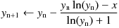
e^W₀(x) — ランベルトの W 関数の主岐の指数 — はニュートン・ラフソン法 (Newton-Raphson method)を使って求めることができます：

$y_\mathrm{n+1} \leftarrow y_\mathrm{n} - \frac{y_\mathrm{n}\ln(y_\mathrm{n}) - x}{\ln(y_\mathrm{n}) + 1}$

また、下記のハレー法 (Halley's method) を使うことも出来ます：

$y_\mathrm{n+1} \leftarrow y_\mathrm{n} + \frac {2y_\mathrm{n}(1 + \ln y_\mathrm{n}) \,(x - y_\mathrm{n} \ln y_\mathrm{n})} {2y_\mathrm{n}(1 + \ln y_\mathrm{n})^2 + x - y_\mathrm{n} \ln y_\mathrm{n}}$

ニュートン・ラフソン法などの反復法を使用して e^W を求める場合、特に 特異点 -1/e に非常に近いときに不適切な初期値を与えると、収束の観点から酷いことになる —収束が遅いばかりでなく他の枝への跳躍も起こりうる— 恐れがあります。したがって初期値は十分良い近似となっているばかりでなく、 特異点で e^W₀ に漸近することが望ましいです。そういった理由で私は初期値を与える近似式として次の式を選びました。この式は e^W₀ の x = -1/e 付近でのピュイズー級数 (Puiseux series) 展開式の第 3項の係数 1/3 を 0.3 で置き換えて第 4項以降を無視したものです。

初期近似

$y_0 = \frac{1}{\mathrm{e}} + \sqrt{\frac{2}{\mathrm{e}} \, \bigg(\frac{1}{\mathrm{e}} + x\bigg)} + 0.3 \,\bigg(\frac{1}{\mathrm{e}} + x\bigg)$

e^W の z = -1/e 付近での級数展開 (Puiseux series) :

$\frac{1}{\mathrm{e}} + \sqrt{\frac{2}{\mathrm{e}}\left(z + \frac{1}{\mathrm{e}}\right)}} +\frac{1}{3} \left(z + \frac{1}{\mathrm{e}}\right) - \frac{1}{18} \sqrt{\frac{\mathrm{e}}{2}} \left(z + \frac{1}{\mathrm{e}}\right)^{\big{\frac{3}{2}}} +O(z^2)$

上記の初期近似式中の係数 0.3 の代わりに、 x = 0 のときに式の値がゼロになる ( e - √2 - 1 ) を使うこともできます。

$y_0 = \frac{1}{\mathrm{e}} + \sqrt{\frac{2}{\mathrm{e}} \, \bigg(\frac{1}{\mathrm{e}} + x\bigg)} + (\mathrm{e} - \sqrt{2} - 1) \,\bigg(\frac{1}{\mathrm{e}} + x\bigg)$

また、ピュイズー級数より、1/3 を使うことも出来ますが、この用途では 0.3 が十分良い値となっています。

次の関係から、ランベルトの W は e^W — ランベルトの W の指数を用いて計算できます。

$W(x) = \frac{x}{\mathrm{e}^{W(x)}} = \ln\big(\mathrm{e}^{W(x)}\big)$

初期近似と収束結果

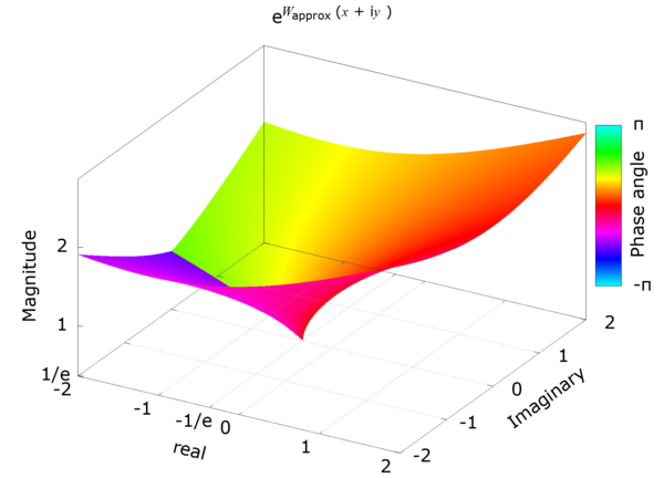
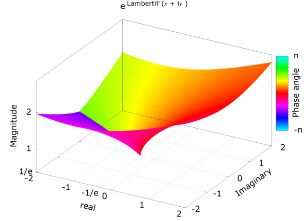
Usage

NAME
     cexplambertw -- exponent of the principal branch of the complex Lambert W function.

LIBRARY
     Math library (libm, -lm)

SYNOPSIS
     #include <math.h>
     #include <complex.h>

     double complex
     cexplambertw(complex double x);

RETURN VALUE
     cexplambertw(x) returns the value of the exponent of the principal branch of the
     complex Lambert W function.

Formulas Used

Iteration formula (Halley's method)

Initial approximation

$y_0 = \frac{1}{\mathrm{e}} + \sqrt{\frac{2}{\mathrm{e}} \, \bigg(\frac{1}{\mathrm{e}} + x\bigg)} + (\mathrm{e} - \sqrt{2} - 1) \,\bigg(\frac{1}{\mathrm{e}} + x\bigg)$

Code (C99)

/* cexplambertw : exponent of Lambert W0 function
    Rev.1.52 (Dec. 4, 2020) (c) Takayuki HOSODA (aka Lyuka)
    http://www.finetune.co.jp/~lyuka/technote/lambertw/
    Acknowledgments: Thanks to Albert Chan for his informative suggestions. 
 */
#include <math.h>
#include <complex.h>

#ifdef HAVE_NO_CLOG
double complex clog(double complex);
double complex clog(double complex x) {
    return log(cabs(x)) + atan2(cimag(x), creal(x)) * I;
}
#endif

double complex cexplambertw(double complex);
double complex cexplambertw(double complex x) {
    double complex y, p, s, t;
    double q, r, m;

    r = 1 / M_E;
    q = M_E - M_SQRT2 - 1;
    if ((fabs(creal(x)) <= (DBL_MAX / 1024.0)) && (fabs(cimag(x)) <= (DBL_MAX / 1024.0))) {
        m = 1.0;
        s = x + r;
        if (s == 0) return r;
        y = (r + csqrt((2.0 * r) * s) + q * s); // approximation near x=-1/e
    } else {
        m = (1.0 / 1024.0);
        x *= m; // scaling
        s = x * m;
        y = r * m + csqrt(r * (s * 64.0)) + q * s;
        y *= 1024.0;
    }
    r = DBL_MAX;
    do {
        q = r; p = y;
        t = clog(y);
        s =  0.5 * (x / y - t * m) / (1 + t) + (1 + t) * m;
        t = (x - y * (t * m));
        y += t / s;
        r = cabs(y - p); // correction radius
    } while (r != 0 && q > r) // convergence check by Urabe's theorem
    return p;
}

cexplambertw() の計算結果の例

cexplambertw(1 - i2) = 1.963022024795711 - i1.157904818620495 (i2.220446049250313e-16)
cexplambertw(1) = 1.763222834351897
cexplambertw(i) = 1.219531415904638 + i0.7927604805362661
cexplambertw(0) = 1
cexplambertw(-0.36) = 0.4466034047150879 (5.551115123125783e-17)
cexplambertw(-0.3678794411714423) = 0.3678794411714423
cexplambertw(-0.37) = 0.3671727690033079 + i0.03950593783033725 (0 - i1.52655665885959e-16)
cexplambertw(-1) = 0.168376379087223 + i0.7077541887847276 (-5.551115123125783e-17 + i0)
cexplambertw(-1.78) = -0.05991375474182515 + i1.091676160700024 (2.081668171172169e-17 + i0)
cexplambertw(-6 + i8) = 0.5264016089780164 + i4.672167782982316 (-1.110223024625157e-16 + i0)
cexplambertw(-1e+40 + i1e+40) = -1.105839096727962e+38 + i1.166002733393464e+38
cexplambertw(1e+99) = 4.493356750426822e+96
cexplambertw(1.797693134862316e+308 + i0) = 2.556348163871691e+305 + i0 (-3.89812560456e+289 + i0)
cexplambertw(-1.797693134862316e+308 + i0) = -2.556297327179282e+305 + i1.140377281032545e+303
cexplambertw(1.797693134862316e+308 + i1.797693134862316e+308) = 2.557935739687931e+305 + i2.552239351260207e+305
cexplambertw(-1.797693134862316e+308 + i1.797693134862316e+308) = -2.546517666521172e+305 + i2.563606662249022e+305 (3.89812560456e+289 + i0)
cexplambertw(0 + i1.797693134862316e+308) = 5.701971348523801e+302 + i2.556335454509411e+305 (7.613526571406249e+286 + i0)

W₀ — ランベルトの W 関数の主枝(principal branch)

特異点を考慮する必要がありますが、 e^W の場合はその値がゼロにならないため、ニュートン・ラフソン法やハレー法で比較的簡単に e^W を求めることができました。しかし、このような反復法で W₀ — ランベルトの W の主枝 — を見つけようとすると、 x がゼロになるときに W₀ もゼロになるため、特異点だけでなくゼロも考慮する必要があります。言い換えると、反復法の初期値の近似式が、特異点とゼロで漸近的に誤差がゼロになることが強く望まれます。また、 W₀ は特異点からの単調増加関数であるため、その近似も単調増加関数である必要があります。これらの要件を満たすために、初期値は次の近似関数を使用して計算されます。

初期近似

$y_0 = \frac{1}{\mathrm{e}} + \sqrt{\frac{2}{\mathrm{e}} \, \bigg(\frac{1}{\mathrm{e}} + x\bigg)} + (\mathrm{e} - \sqrt{2} - 1) \,\bigg(\frac{1}{\mathrm{e}} + x\bigg)$

W₀ は特異点の周りに大きな導関数を持っているため、ニュートン・ラフソン法は、初期近似が不十分な場合、あるいは計算誤差が原因で、特異点の近くで壊滅的な動作を引き起こす可能性があります。したがって、 W₀ を得るためには、ニュートン・ラフソン法よりも特異点近傍での収束性に優れた、ハレー法あるいは 4次のハウスホルダー法 (Householder's method of order 4) を使用します。

ニュートン・ラフソン法

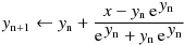
$y_\mathrm{n+1} \leftarrow y_\mathrm{n} + \frac {x - y_\mathrm{n}\, \mathrm{e}^{\, \displaystyle y_\mathrm{n}}} { \mathrm{e}^{\,\displaystyle y_\mathrm{n}} + y_\mathrm{n}\,\mathrm{e}^{\, \displaystyle y_\mathrm{n}}$

ハレー法

$y_\mathrm{n+1} \leftarrow y_\mathrm{n} - \frac {2 (y_\mathrm{n} + 1) \, (y_\mathrm{n}\,\mathrm{e}^{\, \displaystyle y_\mathrm{n}} - x)} { ({ y_\mathrm{n}}^2 + 2 y_\mathrm{n} + 2) \, \mathrm{e}^{\,\displaystyle y_\mathrm{n}} + (y_\mathrm{n} + 2) x}$

4次のハウスホルダー法

$y_{\mathrm n+1} \leftarrow y_{\mathrm n} - \frac{3y_{\mathrm n}^3(\mathrm{e}^{\, \displaystyle y_\mathrm{n}})^2+6y_{\mathrm n}^2(\mathrm{e}^{\, \displaystyle y_\mathrm{n}})^2-3y_{\mathrm n}{x}^2+6y_{\mathrm n}(\mathrm{e}^{\, \displaystyle y_\mathrm{n}})^2-6{x}^2-6{x}\mathrm{e}^{\, \displaystyle y_\mathrm{n}}} {{6y_{\mathrm n}}^2{x}\mathrm{e}^{\, \displaystyle y_\mathrm{n}}+{y_{\mathrm n}}^2\mathrm{e}^{\, \displaystyle y_\mathrm{n}}+18y_{\mathrm n}{x}\mathrm{e}^{\, \displaystyle y_\mathrm{n}}+6y_{\mathrm n}(\mathrm{e}^{\, \displaystyle y_\mathrm{n}})^2+5y_{\mathrm n}\mathrm{e}^{\, \displaystyle y_\mathrm{n}}+12{x}\mathrm{e}^{\, \displaystyle y_\mathrm{n}}+6(\mathrm{e}^{\, \displaystyle y_\mathrm{n}})^2+6\mathrm{e}^{\, \displaystyle y_\mathrm{n}}}$

Usage

NAME
     clambertw -- the principal branch of the complex Lambert W function.

LIBRARY
     Math library (libm, -lm)

SYNOPSIS
     #include <math.h>
     #include <complex.h>

     double complex
     clambertw(complex double x);

RETURN VALUE
     clambertw(x) returns complex value of the principal branch
     of the Lambert W function.

Formulas Used

Iteration formula (Halley's method)

Initial approximation

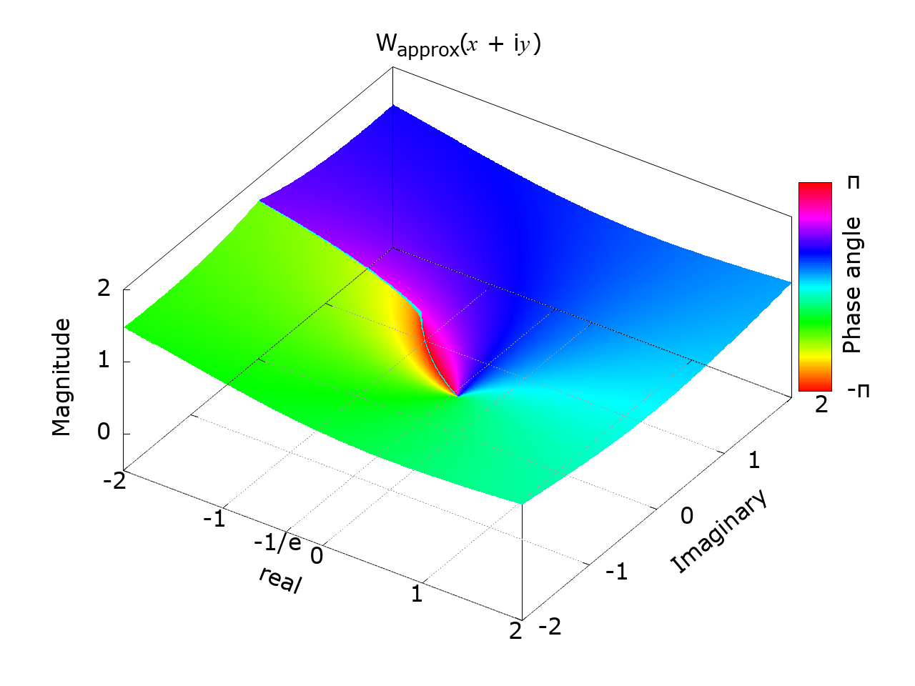
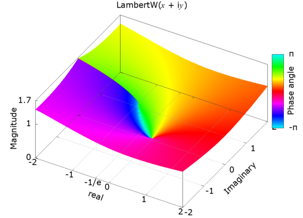
$y_0 = \ln\left(\frac{1}{\mathrm{e}} + \sqrt{\frac{2}{\mathrm{e}} \, \left(\frac{1}{\mathrm{e}} + x\right)} + (\mathrm{e} - \sqrt{2} - 1) \,\left(\frac{1}{\mathrm{e}} + x\right)\right)$

Initial approximation and refined result

Code (C99)

/* clambertw : Lambert W0 function 
    Rev.1.52 (Dec. 4, 2020) (c) Takayuki HOSODA (aka Lyuka)
    http://www.finetune.co.jp/~lyuka/technote/lambertw/
    Acknowledgments: Thanks to Albert Chan for his informative suggestions.
 */
#include <math.h>
#include <complex.h>
#include <float.h>

#ifdef HAVE_NO_CLOG
double complex clog(double complex);
double complex clog(double complex x) {
    return log(cabs(x)) + atan2(cimag(x), creal(x)) * I;
}
#endif

double complex clambertw(double complex);
double complex clambertw(double complex x) {
    double complex y, p, s, t;
    double q, r, m;

    r = 1 / M_E;
    q = M_E - M_SQRT2 - 1;
    if ((fabs(creal(x)) <= (DBL_MAX / 1024.0)) && (fabs(cimag(x)) <= (DBL_MAX / 1024.0))) {
        m = 1.0;
        s = x + r;
        if (s == 0) return -1;
        y = clog(r + csqrt((2.0 * r) * s) + q * s); // approximation near x=-1/e
    } else {
        m = (1.0 / 1024.0);
        x *= m; // scaling
        s = x * m;
        y = clog(r * m + csqrt(r * (s * 64.0)) + q * s);
        y += (M_LN2 * 10.0);
    }
    r = DBL_MAX;
    do {
        q = r; p = y;
        t = cexp(y) * m;
        s = y * t - x;
        u = (0.5 * y) / (y + 1.0) * s + t + x;
        y -= s / u // Halley's method
        r = cabs(y - p); // correction radius
    } while (r != 0 && q > r); // convergence check by Urabe's theorem
    return p;
}

clambertw() の計算結果の例

clambertw(2.718281828459045 + i0) = 0.9999999999999999 + i0 (1.110223024625157e-16 + i0)
clambertw(1 - i2) = 0.8237712167092305 - i0.5329289867954415 (0 - i1.110223024625157e-16)
clambertw(1 + i0) = 0.5671432904097838 + i0
clambertw(0 + i1) = 0.3746990207371175 + i0.5764127230314353 (-5.551115123125783e-17 + i0)
clambertw(0 + i0) = 0 + i0
clambertw(-0.36 + i0) = -0.8060843159708175 + i0 (-2.220446049250313e-16 + i0)
clambertw(-0.3678794411714423 + i0) = -1 + i0
clambertw(-0.37 + i0) = -0.996167692712445 + i0.1071826188083488 (3.33066907387547e-16 + i1.956768080901838e-15)
clambertw(-1 + i0) = -0.3181315052047642 + i1.337235701430689 (1.110223024625157e-16 + i2.220446049250313e-16)
clambertw(-1.78 + i0) = 0.08921804985620939 + i1.625623674427768 (-6.938893903907228e-17 + i0)
clambertw(-6 + i8) = 1.547930197079636 + i1.458601930168348
clambertw(-1e+40 + i1e+40) = 87.9726013585729 + i2.329718360883123
clambertw(1e+99 + i0) = 222.5507689557502 + i0
clambertw(1.797693134862316e+308 + i0) = 703.2270331047702 + i0
clambertw(-1.797693134862316e+308 + i0) = 703.2270231685106 + i3.137131632158036
clambertw(0 + i1.797693134862316e+308) = 703.2270306206868 + i1.568565805021136
clambertw(-1.797693134862316e+308 + i1.797693134862316e+308) = 703.5731090989279 + i2.352850357853284
clambertw(1.797693134862316e+308 + i1.797693134862316e+308) = 703.5731140622003 + i0.7842834489371958

WolframAlpha による計算結果の例

W₀(e) = 1
W₀(1 ± i2) ≈0.823771216709230498962714234680902867860235005053071922240368278… ± i0.532928986795441605088201422572330085339330393308596795767937866…
W₀(1) ≈ 0.5671432904097838729999686622103555497538157871865125081351310792…
W₀(i) ≈ 0.374699020737117493605978428759720807512802175326782642557502432… + i0.576412723031435283148289239887068476278099011222168280566265741…
W₀(0) = 0
W₀(-0.36) ≈ -0.806084315970817778285521361620992001997459968346671301630…
W₀(-1 / e) = -1
W₀(-0.37) ≈ -0.99616769271244462673848201201414760619715183596966610666601412… + i0.10718261880835079146468624812898507138565644109822599338982371…
W₀(-1) ≈ -0.31813150520476413531265425158766451720351761387139986692237860… + i1.3372357014306894089011621431937106125395021384605124188763127…
W₀(-1.78) ≈ 0.089218049856209317716109060765294251305387407793167833503833064… + i1.6256236744277681331520891017303249073577948841857860157186500…
W₀(-6 ± i8) ≈ 1.547930197079635814768631631342423213473126810818780368642414024… ± i1.458601930168348176634851154910250705430582638721325124179334991…
W₀(-1e40 ± i1e40) ≈ 87.97260135857290602332406004222549277677935447060989442026705176… ± i2.329718360883123170160790314772387815611852082396629087352292852…
W₀(1e99) ≈ 222.55076895575017934955228965217449610853244528249943629448650570…
W₀(1e305) ≈ 695.74347234500662968414578760461819217555667677555452851562125354…
W₀(1e305 ± i1e305) ≈ 696.089548005772131650126785445013705743509108054188263218466334… ± i0.784271481992182658322800157708303004261113225909172777370356203…

追補

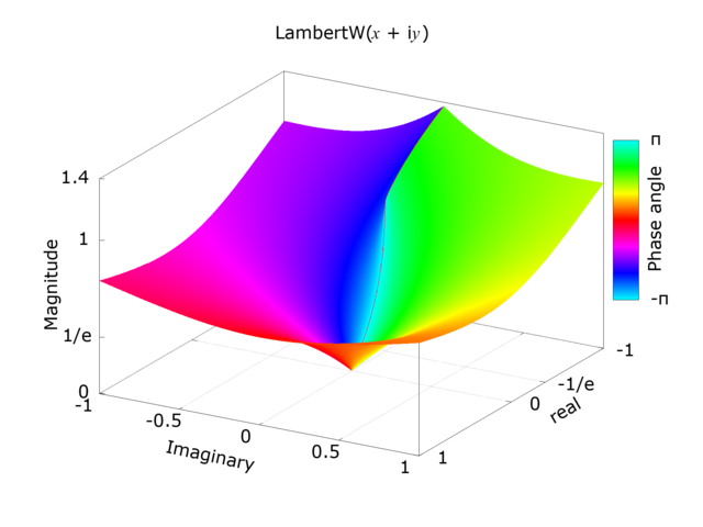
gnuplot の splot と pm3d を使った、複素ランベルトの W の 4Dプロットの例 — プロット用スクリプトとデータと参考画像

ダウンロード : lambertw-gnuplot-pm3d.zip [1MB zip]

参考文献

以下の参考文献は、ランベルトのW関数、ピュイズー級数、および数値反復法に関する一般的な背景情報を提供しています。

Lambert W function: "Lambert W-function", Wolfram MathWorld
Numerical methods: "Newton's Method", Wolfram MathWorld
Numerical methods: "Householder's Method", Wolfram MathWorld
Background: "Why W?", Hayes, B. (2005). American Scientist. 93 (2): 104‐108.
Lambert W overview: "The Lambert W function poster", ORCCA
Convergence theory: "Convergence of Numerical Iteration in Solution of Equations", M. Urabe, J. Sci. Hiroshima Univ. Ser. A, 19 (3), 1956.
Floating-point / numerical robustness: "Mathematics Written in Sand", W. Kahan, 1983.
Complex arithmetic: "Improved Complex Division", Baudin & Smith
General references: Wikipedia — Lambert W function
General references: Wikipedia — Puiseux series
Libraries: GNU Scientific Library
Visualization: gnuplot pm3d demo

概要

eW0 — ランベルトの W 関数の主岐の指数

反復法

初期近似

初期近似と収束結果

Usage

Formulas Used

Iteration formula (Halley's method)

Initial approximation

Code (C99)

cexplambertw() の計算結果の例

W0 — ランベルトの W 関数の主枝(principal branch)

初期近似

ニュートン・ラフソン法

ハレー法

4次のハウスホルダー法

Usage

Formulas Used

Iteration formula (Halley's method)

Initial approximation

Initial approximation and refined result

Code (C99)

clambertw() の計算結果の例

WolframAlpha による計算結果の例

追補

参考文献

関連項目

e^W₀ — ランベルトの W 関数の主岐の指数

W₀ — ランベルトの W 関数の主枝(principal branch)