Overview
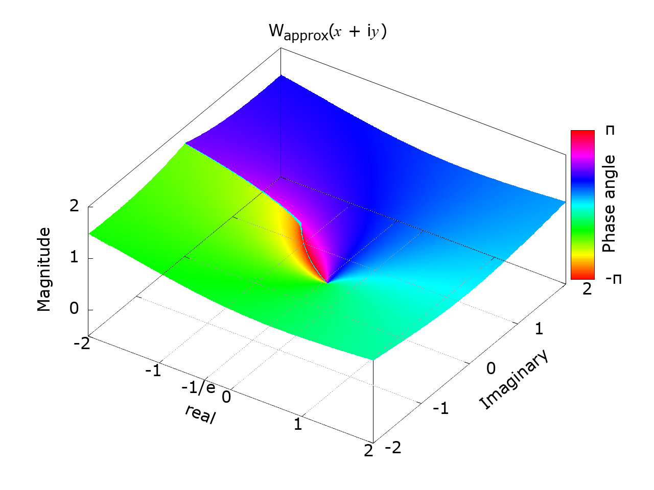
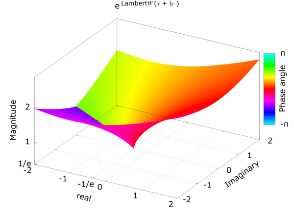
This is an implementation of the complex Lambert W-function and its exponential function, utilizing an initial approximation by Puiseux and Halley's iterative method optimized for the HP Prime CAS environment.
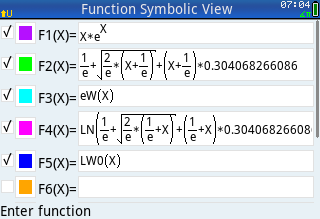
Implementation of W0(x)
Usage
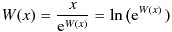
LW0C(x) — calculate the principal branch of the Lambert W function.Formulas used
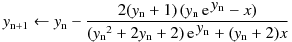
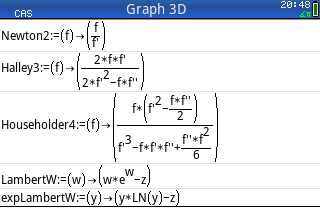
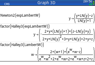
Recurrence formula (Halley's method):
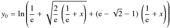
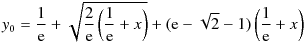
Initial approximation:
Code
LW0C Rev.1.52 (Dec. 4, 2020)#CAS
//LW0C - Principal branch of the Lambert W function
//Rev.1.52 (Dec. 4, 2020) (c) Takayuki HOSODA (aka Lyuka)
//Acknowledgments: Thanks to Albert Chan for his informative suggestions.
LW0C(x):=
BEGIN
LOCAL y, p, s, t;
LOCAL q, r, m;
HComplex := 1; // Enable complex result from a real input.
r := 1.0 / e;
q := e - sqrt(2.0) - 1.0;
m := MAXREAL / 1024.0;
IF abs(RE(x)) <= m AND abs(IM(x)) <= m THEN
m := 1.0;
s := x + r;
IF s == 0 THEN return -1; END;
y := ln(r + sqrt(2.0 * r * s) + q * s); // approximation near x=-1/e
ELSE
m := 1.0 / 1024.0;
x := x * m;
s := x * m;
y := ln(r * m + sqrt(r * (s * 64.0)) + q * s);
y := y + 6.931471805599453094; // + ln(2) * 10
END;
r := MAXREAL; //1.79769313486e308
REPEAT
q := r;
p := y;
t := exp(y) * m;
s := y * t - x;
t := (0.5 * y) * inv(y + 1.0) * s + t + x; // t <> 0
y := y - s * inv(t); // Halley's method
r := abs(y - p); // correction radius;
UNTIL 0 == r OR q <= r; // convergence check
return p;
END;
#END
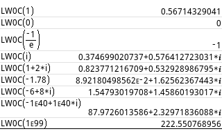
Calculation example of LW0C
Implementation of eW0(x)
Usage
eW(x) — calculate the exponent of the principal branch of the Lambert W function.Formulas used
Recurrence formula (Halley's method):
Initial approximation:
From the relation below,the Lambert W0 can be obtained from the relation:
Code
eW Rev.1.52 (Dec. 4, 2020)#CAS
//eW : exponent of the Lambert W0 function
//Rev.1.52 (Dec. 4, 2020) (c) Takayuki HOSODA (aka Lyuka)
// http://www.finetune.co.jp/~lyuka/technote/lambertw/
//Acknowledgments: Thanks to Albert Chan for his informative suggestions.
eW(x):=
BEGIN
LOCAL y, p, s, t, u, v;
LOCAL q, r, m;
HComplex := 1; // Enable complex result from a real input.
r := 1.0 / e;
q := e - sqrt(2) - 1;
s := x + r;
IF s == 0 THEN return r; END;
m := MAXREAL / 1024.0;
IF abs(RE(x)) <= m AND abs(IM(x)) <= m THEN
m := 1.0;
y := r + sqrt(2.0 * r * s) + q * s; // approximation near x=-1/e
ELSE
m := 1.0 / 1024.0;
x := x * m;
s := x * m;
y := r * m + sqrt(r * (s * 64.0)) + q * s;
y := y * 1024.0;
END;
r := MAXREAL;
REPEAT
q := r;
p := y;
t := ln(y);
v := 1 + t;
s := 0.5 * (x * inv(y) - t * m) * inv(v) + v * m; //s <> 0, y <> 0, v <> 0
t := (x - y * (t * m));
y := y + t * inv(s); // Halley's method
r := cabs(y - p); // correction radius
UNTIL 0 == r OR q <= r; // convergence check
return p;
END;
// This is a workaround for the dynamic range problem of complex division and abs() in CAS.
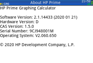
// Conforms to HP Prime software version 2.1.14433 (2020 01 21).
// cabs(z) -- returns the magnitude of the complex number z.
cabs(z):=
BEGIN
LOCAL x, y, t, s;
x := RE(z);
y := IM(z);
IF x < 0 THEN x := -x; END;
IF y < 0 THEN y := -y; END;
IF x == 0 THEN return y; END;
IF y == 0 THEN return x; END;
IF (y > x) THEN
t := x; x := y; y := t;
END;
t := x - y;
IF t > y THEN
t := x / y;
t := t + sqrt(1 + t * t);
ELSE
t := t / y;
s := t * (t + 2);
t := t + s / (sqrt(2) + sqrt(2 + s));
t := t + sqrt(2) + 1;
END;
return(x + y / t);
END;
#END
Householder's method (order 4) — a Higher-order iteration
As an experimental extension, a higher-order iteration (Householder's method of order 4) is applied using the same Puiseux-based initial approximation.
This serves to assess the practical robustness of the initial approximation beyond Halley's method, based on its structural consistency with the underlying function. In particular, the initial approximation incorporates the local Puiseux-series structure near the branch point and matches the behavior at both x = 0 and x = -1/e, providing a consistent starting value.
Although the method achieves higher-order asymptotic convergence, its advantage diminishes under finite-precision arithmetic, and its practical performance on HP Prime is limited by computational overhead. Empirically, stable convergence is observed even for higher-order iterations.
Usage
LW0H(x) — calculate the principal branch of the Lambert W function.Formulas used
Recurrence formula (Householder's method of order 4):

Initial approximation:
Code
This implementation is provided for comparison with Halley's method, using the same initial approximation.
LW0H Rev.1.46 (Nov. 28, 2020)#CAS
//LW0H - Principal branch of the Lambert W function
//Rev.1.46 (Nov. 28, 2020) (c) Takayuki HOSODA (aka Lyuka)
//Acknowledgments: Thanks to Albert Chan for his informative suggestions.
LW0H(x):=
BEGIN
LOCAL y, p, s, t, u, v;
LOCAL q, r;
HComplex := 1; // Enable complex result from a real input.
r := sqrt(MAXREAL) / 1e4; // Limit x range
IF abs(RE(x)) > r OR abs(IM(x)) > r THEN return "LW0H: x out of range"; END;
r := 1.0 / e;
s := x + r;
IF s == 0 THEN return -1; END;
q := e - sqrt(2.0) - 1.0;
y := 1.0 * ln(r + sqrt(2.0 * r * s) + q * s); // approximation near x=-1/e
r := MAXREAL;
REPEAT
q := r;
p := y;
s := exp(y);
t := s + x;
u := y * s;
v := u - x;
v := (6.0 * ((y + 1.0) * u * x + t * (t + u)) + v * (3.0 * (u + x) + y * v));
IF (0 == v) THEN break; END;
t := 3.0 * (u - x) * ((u + x) * (y + 2.0) + 2.0 * s);
y := y - t * inv(v); // Householder's method of order 4
r := abs(y - p); // correction radius
UNTIL 0 == r OR q <= r; // convergence check by Urabe's theorem
return p;
END;
#END
Practical performance on HP Prime
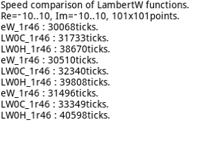
The higher-order iteration converges reliably with the same initial approximation, but does not provide a performance advantage on HP Prime.
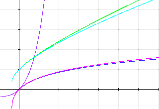
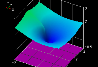
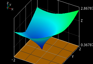
Visualization on HP Prime (3D plot reproduction)
Reference
- Lambert W function: "Lambert W-function", Wolfram MathWorld
- Numerical methods: "Newton's Method", Wolfram MathWorld
- Numerical methods: "Householder's Method", Wolfram MathWorld
- Background: "Why W?", Hayes, B. (2005). American Scientist. 93 (2): 104‐108.
- Lambert W overview: "The Lambert W function poster", ORCCA
- Convergence theory: "Convergence of Numerical Iteration in Solution of Equations", M. Urabe, J. Sci. Hiroshima Univ. Ser. A, 19 (3), 1956.
- Floating-point / numerical robustness: "Mathematics Written in Sand", W. Kahan, 1983.
- Complex arithmetic: "Improved Complex Division", Baudin & Smith
- General references: Wikipedia — Lambert W function
- General references: Wikipedia — Puiseux series
- Libraries: GNU Scientific Library
- Visualization: gnuplot pm3d demo