Branch-Stable Evaluation of the Lambert W Function (W<sub>0</sub>) Using Puiseux-Series Initial Approximation

Overview

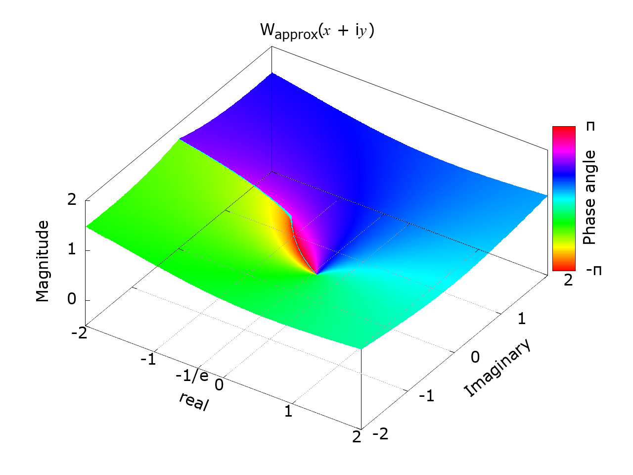
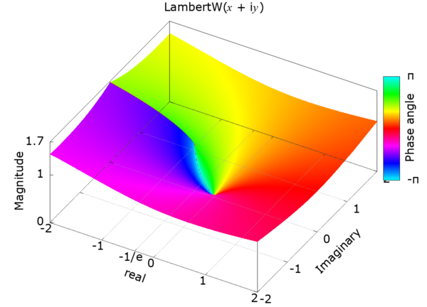
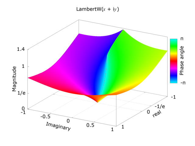
The Lambert W function, defined as the inverse of f(w) = we^w, is a multi-valued function in the complex domain. Its principal branch W₀ is the branch that remains real-valued for real inputs x ≥ -1/e, and is widely used in numerical applications.

In practical implementations, however, evaluating W₀ is not trivial. Iterative methods such as Halley's method provide fast convergence, but their behavior strongly depends on the initial approximation. A poor initial guess can lead to convergence to an unintended branch, especially for complex arguments near the branch point.

This page presents a branch-stable approach based on a Puiseux-series initial approximation around the critical region. By capturing the local structure of the function, the method provides reliable initial values that enable stable and consistent convergence of Halley iteration to the principal branch W₀.

Implementation examples in C99 are provided to demonstrate a practical realization of the method.

W₀ — Principal branch and numerical issues

The principal branch W₀ of the Lambert W function is defined for complex arguments and plays a central role in numerical applications. However, its evaluation is nontrivial due to the presence of a branch point at x = -1/e, where the derivative becomes large and the function exhibits square-root-type behavior.

Iterative methods such as Newton–Raphson or Halley iteration can achieve rapid convergence, but their stability critically depends on the initial approximation. A poor initial guess may lead to convergence to an unintended branch, especially in the complex domain near the branch point.

To address this issue, the initial value is constructed using a Puiseux-series-based approximation that captures the local structure around the branch point. This provides a branch-consistent starting point and ensures stable convergence to W₀.

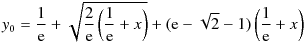
The following approximation is used as the initial estimate. It is constructed from a truncated Puiseux expansion around the branch point x = -1/e, and the coefficients are further adjusted so that the approximation satisfies W₀(0) = 0. This effectively provides consistency at both the branch point and the origin.

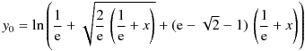
$y_0 = \frac{1}{\mathrm{e}} + \sqrt{\frac{2}{\mathrm{e}} \, \bigg(\frac{1}{\mathrm{e}} + x\bigg)} + (\mathrm{e} - \sqrt{2} - 1) \,\bigg(\frac{1}{\mathrm{e}} + x\bigg)$

The role of the initial approximation is to ensure branch-consistent convergence; the final accuracy is obtained by iterative refinement.

Newton–Raphson iteration is shown for reference, although it may exhibit unstable behavior near the branch point.

Newton–Raphson method: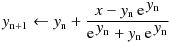

$y_\mathrm{n+1} \leftarrow y_\mathrm{n} + \frac {x - y_\mathrm{n}\, \mathrm{e}^{\, \displaystyle y_\mathrm{n}}} { \mathrm{e}^{\,\displaystyle y_\mathrm{n}} + y_\mathrm{n}\,\mathrm{e}^{\, \displaystyle y_\mathrm{n}}$

Halley's method is used as the primary iteration due to its cubic convergence and robustness.

Halley's method: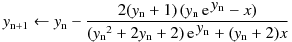

$y_\mathrm{n+1} \leftarrow y_\mathrm{n} - \frac {2 (y_\mathrm{n} + 1) \, (y_\mathrm{n}\,\mathrm{e}^{\, \displaystyle y_\mathrm{n}} - x)} { ({ y_\mathrm{n}}^2 + 2 y_\mathrm{n} + 2) \, \mathrm{e}^{\,\displaystyle y_\mathrm{n}} + (y_\mathrm{n} + 2) x}$

For reference, a higher-order iteration such as Householder's method (order 4) can also be applied, although such schemes tend to be more sensitive to the initial approximation in the complex domain.

Householder's method of order 4:

$y_{\mathrm n+1} \leftarrow y_{\mathrm n} - \frac{3y_{\mathrm n}^3(\mathrm{e}^{\, \displaystyle y_\mathrm{n}})^2+6y_{\mathrm n}^2(\mathrm{e}^{\, \displaystyle y_\mathrm{n}})^2-3y_{\mathrm n}{x}^2+6y_{\mathrm n}(\mathrm{e}^{\, \displaystyle y_\mathrm{n}})^2-6{x}^2-6{x}\mathrm{e}^{\, \displaystyle y_\mathrm{n}}} {{6y_{\mathrm n}}^2{x}\mathrm{e}^{\, \displaystyle y_\mathrm{n}}+{y_{\mathrm n}}^2\mathrm{e}^{\, \displaystyle y_\mathrm{n}}+18y_{\mathrm n}{x}\mathrm{e}^{\, \displaystyle y_\mathrm{n}}+6y_{\mathrm n}(\mathrm{e}^{\, \displaystyle y_\mathrm{n}})^2+5y_{\mathrm n}\mathrm{e}^{\, \displaystyle y_\mathrm{n}}+12{x}\mathrm{e}^{\, \displaystyle y_\mathrm{n}}+6(\mathrm{e}^{\, \displaystyle y_\mathrm{n}})^2+6\mathrm{e}^{\, \displaystyle y_\mathrm{n}}}$

Implementation examples in C99

Usage

NAME
     clambertw -- the principal branch of the complex Lambert W function.

LIBRARY
     Math library (libm, -lm)

SYNOPSIS
     #include <math.h>
     #include <complex.h>

     double complex
     clambertw(complex double x);

RETURN VALUE
     clambertw(x) returns complex value of the principal branch
     of the Lambert W function.

Formulas Used

Iteration formula (Halley's method):

Initial approximation:

$y_0 = \ln\left(\frac{1}{\mathrm{e}} + \sqrt{\frac{2}{\mathrm{e}} \, \left(\frac{1}{\mathrm{e}} + x\right)} + (\mathrm{e} - \sqrt{2} - 1) \,\left(\frac{1}{\mathrm{e}} + x\right)\right)$

Initial approximation and refined result

The initial approximation captures the local structure near the branch point, providing a stable starting point for branch-consistent convergence.

Code (C99)

/* clambertw : Lambert W0 function 
    Rev.1.52 (Dec. 4, 2020) (c) Takayuki HOSODA (aka Lyuka)
    http://www.finetune.co.jp/~lyuka/technote/lambertw/
    Acknowledgments: Thanks to Albert Chan for his informative suggestions.
 */
#include <math.h>
#include <complex.h>
#include <float.h>

#ifdef HAVE_NO_CLOG
double complex clog(double complex);
double complex clog(double complex x) {
    return log(cabs(x)) + atan2(cimag(x), creal(x)) * I;
}
#endif

double complex clambertw(double complex);
double complex clambertw(double complex x) {
    double complex y, p, s, t;
    double q, r, m;

    r = 1 / M_E;
    q = M_E - M_SQRT2 - 1;
    if ((fabs(creal(x)) <= (DBL_MAX / 1024.0)) && (fabs(cimag(x)) <= (DBL_MAX / 1024.0))) {
        m = 1.0;
        s = x + r;
        if (s == 0) return -1;
        y = clog(r + csqrt((2.0 * r) * s) + q * s); // approximation near x=-1/e
    } else {
        m = (1.0 / 1024.0);
        x *= m; // scaling
        s = x * m;
        y = clog(r * m + csqrt(r * (s * 64.0)) + q * s);
        y += (M_LN2 * 10.0);
    }
    r = DBL_MAX;
    do {
        q = r; p = y;
        t = cexp(y) * m;
        s = y * t - x;
        u = (0.5 * y) / (y + 1.0) * s + t + x;
        y -= s / u // Halley's method
        r = cabs(y - p); // correction radius
    } while (r != 0 && q > r); // convergence check by Urabe's theorem
    return p;
}

Calculation example of clambertw()

Calculation results — `clambertw()`

clambertw(2.718281828459045 + i0) = 0.9999999999999999 + i0 (1.110223024625157e-16 + i0)
clambertw(1 - i2) = 0.8237712167092305 - i0.5329289867954415 (0 - i1.110223024625157e-16)
clambertw(1 + i0) = 0.5671432904097838 + i0
clambertw(0 + i1) = 0.3746990207371175 + i0.5764127230314353 (-5.551115123125783e-17 + i0)
clambertw(0 + i0) = 0 + i0
clambertw(-0.36 + i0) = -0.8060843159708175 + i0 (-2.220446049250313e-16 + i0)
clambertw(-0.3678794411714423 + i0) = -1 + i0
clambertw(-0.37 + i0) = -0.996167692712445 + i0.1071826188083488 (3.33066907387547e-16 + i1.956768080901838e-15)
clambertw(-1 + i0) = -0.3181315052047642 + i1.337235701430689 (1.110223024625157e-16 + i2.220446049250313e-16)
clambertw(-1.78 + i0) = 0.08921804985620939 + i1.625623674427768 (-6.938893903907228e-17 + i0)
clambertw(-6 + i8) = 1.547930197079636 + i1.458601930168348
clambertw(-1e+40 + i1e+40) = 87.9726013585729 + i2.329718360883123
clambertw(1e+99 + i0) = 222.5507689557502 + i0
clambertw(1.797693134862316e+308 + i0) = 703.2270331047702 + i0
clambertw(-1.797693134862316e+308 + i0) = 703.2270231685106 + i3.137131632158036
clambertw(0 + i1.797693134862316e+308) = 703.2270306206868 + i1.568565805021136
clambertw(-1.797693134862316e+308 + i1.797693134862316e+308) = 703.5731090989279 + i2.352850357853284
clambertw(1.797693134862316e+308 + i1.797693134862316e+308) = 703.5731140622003 + i0.7842834489371958

Calculation results — WolframAlpha

W₀(e) = 1
W₀(1 ± i2) ≈0.823771216709230498962714234680902867860235005053071922240368278… ± i0.532928986795441605088201422572330085339330393308596795767937866…
W₀(1) ≈ 0.5671432904097838729999686622103555497538157871865125081351310792…
W₀(i) ≈ 0.374699020737117493605978428759720807512802175326782642557502432… + i0.576412723031435283148289239887068476278099011222168280566265741…
W₀(0) = 0
W₀(-0.36) ≈ -0.806084315970817778285521361620992001997459968346671301630…
W₀(-1 / e) = -1
W₀(-0.37) ≈ -0.99616769271244462673848201201414760619715183596966610666601412… + i0.10718261880835079146468624812898507138565644109822599338982371…
W₀(-1) ≈ -0.31813150520476413531265425158766451720351761387139986692237860… + i1.3372357014306894089011621431937106125395021384605124188763127…
W₀(-1.78) ≈ 0.089218049856209317716109060765294251305387407793167833503833064… + i1.6256236744277681331520891017303249073577948841857860157186500…
W₀(-6 ± i8) ≈ 1.547930197079635814768631631342423213473126810818780368642414024… ± i1.458601930168348176634851154910250705430582638721325124179334991…
W₀(-1e40 ± i1e40) ≈ 87.97260135857290602332406004222549277677935447060989442026705176… ± i2.329718360883123170160790314772387815611852082396629087352292852…
W₀(1e99) ≈ 222.55076895575017934955228965217449610853244528249943629448650570…
W₀(1e305) ≈ 695.74347234500662968414578760461819217555667677555452851562125354…
W₀(1e305 ± i1e305) ≈ 696.089548005772131650126785445013705743509108054188263218466334… ± i0.784271481992182658322800157708303004261113225909172777370356203…

Exponent of the principal branch of the Lambert `W` function

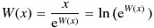
Instead of solving directly for W₀(x), it is sometimes advantageous to consider y = e^W₀(x). From the defining relation W e^W = x, this leads to the equation y ln(y) = x.

This formulation avoids the explicit evaluation of W during iteration and can offer improved numerical stability, especially near the branch point x = -1/e.

The value of y can be obtained by iterative methods such as Newton–Raphson or Halley iteration:

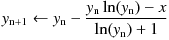
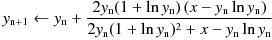
$y_\mathrm{n+1} \leftarrow y_\mathrm{n} - \frac{y_\mathrm{n}\ln(y_\mathrm{n}) - x}{\ln(y_\mathrm{n}) + 1}$

Alternatively, Halley's method can be used:

$y_\mathrm{n+1} \leftarrow y_\mathrm{n} + \frac {2y_\mathrm{n}(1 + \ln y_\mathrm{n}) \,(x - y_\mathrm{n} \ln y_\mathrm{n})} {2y_\mathrm{n}(1 + \ln y_\mathrm{n})^2 + x - y_\mathrm{n} \ln y_\mathrm{n}}$

As with W₀, the convergence depends strongly on the initial approximation. To ensure branch-consistent convergence, the initial value is constructed based on the Puiseux expansion around the branch point x = -1/e.

Starting from the Puiseux series expansion of e^W₀, we truncate the series after the linear term. The resulting approximation already captures the local structure near the branch point.

Series expansion of e^W at z = -1/e (Puiseux series):

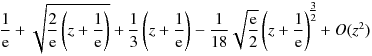
$\frac{1}{\mathrm{e}} + \sqrt{\frac{2}{\mathrm{e}}\left(z + \frac{1}{\mathrm{e}}\right)}} +\frac{1}{3} \left(z + \frac{1}{\mathrm{e}}\right) - \frac{1}{18} \sqrt{\frac{\mathrm{e}}{2}} \left(z + \frac{1}{\mathrm{e}}\right)^{\big{\frac{3}{2}}} +O(z^2)$

To improve global consistency, the linear coefficient is adjusted so that y = 1 at x = 0, which matches the exact value e^W₀(0) = 1.

This yields the following initial approximation:

$y_0 = \frac{1}{\mathrm{e}} + \sqrt{\frac{2}{\mathrm{e}} \, \bigg(\frac{1}{\mathrm{e}} + x\bigg)} + (\mathrm{e} - \sqrt{2} - 1) \,\bigg(\frac{1}{\mathrm{e}} + x\bigg)$

Once y = e^W(x) is obtained, the Lambert W function can be recovered as

$W(x) = \frac{x}{\mathrm{e}^{W(x)}} = \ln\big(\mathrm{e}^{W(x)}\big)$

Usage

NAME
     cexplambertw -- exponent of the principal branch of the complex Lambert W function.

LIBRARY
     Math library (libm, -lm)

SYNOPSIS
     #include <math.h>
     #include <complex.h>

     double complex
     cexplambertw(complex double x);

RETURN VALUE
     cexplambertw(x) returns the value of the exponent of the principal branch of the complex Lambert W function.

Formulas Used

Iteration formula (Halley's method):

Initial approximation:

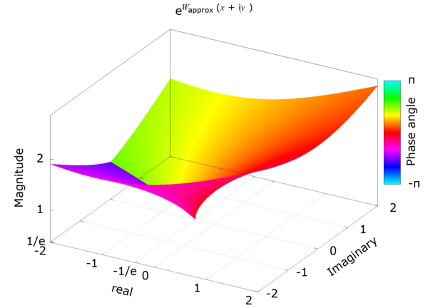
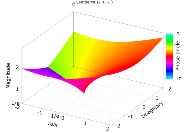
$y_0 = \frac{1}{\mathrm{e}} + \sqrt{\frac{2}{\mathrm{e}} \, \bigg(\frac{1}{\mathrm{e}} + x\bigg)} + (\mathrm{e} - \sqrt{2} - 1) \,\bigg(\frac{1}{\mathrm{e}} + x\bigg)$

Initial approximation and refined result

Code (C99)

/* cexplambertw : exponent of Lambert W0 function
    Rev.1.52 (Dec. 4, 2020) (c) Takayuki HOSODA (aka Lyuka)
    http://www.finetune.co.jp/~lyuka/technote/lambertw/
    Acknowledgments: Thanks to Albert Chan for his informative suggestions. 
 */
#include <math.h>
#include <complex.h>

#ifdef HAVE_NO_CLOG
double complex clog(double complex);
double complex clog(double complex x) {
    return log(cabs(x)) + atan2(cimag(x), creal(x)) * I;
}
#endif

double complex cexplambertw(double complex);
double complex cexplambertw(double complex x) {
    double complex y, p, s, t;
    double q, r, m;

    r = 1 / M_E;
    q = M_E - M_SQRT2 - 1;
    if ((fabs(creal(x)) <= (DBL_MAX / 1024.0)) && (fabs(cimag(x)) <= (DBL_MAX / 1024.0))) {
        m = 1.0;
        s = x + r;
        if (s == 0) return r;
        y = (r + csqrt((2.0 * r) * s) + q * s); // approximation near x=-1/e
    } else {
        m = (1.0 / 1024.0);
        x *= m; // scaling
        s = x * m;
        y = r * m + csqrt(r * (s * 64.0)) + q * s;
        y *= 1024.0;
    }
    r = DBL_MAX;
    do {
        q = r; p = y;
        t = clog(y);
        s =  0.5 * (x / y - t * m) / (1 + t) + (1 + t) * m;
        t = (x - y * (t * m));
        y += t / s;
        r = cabs(y - p); // correction radius
    } while (r != 0 && q > r) // convergence check by Urabe's theorem
    return p;
}

Calculation example — cexplambertw

cexplambertw(1 - i2) = 1.963022024795711 - i1.157904818620495 (i2.220446049250313e-16)
cexplambertw(1) = 1.763222834351897
cexplambertw(i) = 1.219531415904638 + i0.7927604805362661
cexplambertw(0) = 1
cexplambertw(-0.36) = 0.4466034047150879 (5.551115123125783e-17)
cexplambertw(-0.3678794411714423) = 0.3678794411714423
cexplambertw(-0.37) = 0.3671727690033079 + i0.03950593783033725 (0 - i1.52655665885959e-16)
cexplambertw(-1) = 0.168376379087223 + i0.7077541887847276 (-5.551115123125783e-17 + i0)
cexplambertw(-1.78) = -0.05991375474182515 + i1.091676160700024 (2.081668171172169e-17 + i0)
cexplambertw(-6 + i8) = 0.5264016089780164 + i4.672167782982316 (-1.110223024625157e-16 + i0)
cexplambertw(-1e+40 + i1e+40) = -1.105839096727962e+38 + i1.166002733393464e+38
cexplambertw(1e+99) = 4.493356750426822e+96
cexplambertw(1.797693134862316e+308 + i0) = 2.556348163871691e+305 + i0 (-3.89812560456e+289 + i0)
cexplambertw(-1.797693134862316e+308 + i0) = -2.556297327179282e+305 + i1.140377281032545e+303
cexplambertw(1.797693134862316e+308 + i1.797693134862316e+308) = 2.557935739687931e+305 + i2.552239351260207e+305
cexplambertw(-1.797693134862316e+308 + i1.797693134862316e+308) = -2.546517666521172e+305 + i2.563606662249022e+305 (3.89812560456e+289 + i0)
cexplambertw(0 + i1.797693134862316e+308) = 5.701971348523801e+302 + i2.556335454509411e+305 (7.613526571406249e+286 + i0)

Appendix

4D plot of complex LambertW using gnuplot splot with pm3d -- Plot scripts, data and reference images.

Download: lambertw-gnuplot-pm3d.zip [5MB zip]

References

The following references provide general background on the Lambert W function, Puiseux series, and numerical iteration methods.

Lambert W function: "Lambert W-function", Wolfram MathWorld
Numerical methods: "Newton's Method", Wolfram MathWorld
Numerical methods: "Householder's Method", Wolfram MathWorld
Background: "Why W?", Hayes, B. (2005). American Scientist. 93 (2): 104‐108.
Lambert W overview: "The Lambert W function poster", ORCCA
Convergence theory: "Convergence of Numerical Iteration in Solution of Equations", M. Urabe, J. Sci. Hiroshima Univ. Ser. A, 19 (3), 1956.
Floating-point / numerical robustness: "Mathematics Written in Sand", W. Kahan, 1983.
Complex arithmetic: "Improved Complex Division", Baudin & Smith
General references: Wikipedia — Lambert W function
General references: Wikipedia — Puiseux series
Libraries: GNU Scientific Library
Visualization: gnuplot pm3d demo

Branch-Stable Evaluation of the Lambert W Function (W₀) Using Puiseux-Series Initial Approximation

Overview

W₀ — Principal branch and numerical issues

Implementation examples in C99

Usage

Formulas Used

Initial approximation and refined result

Code (C99)

Calculation example of clambertw()

Calculation results — `clambertw()`

Calculation results — WolframAlpha

Exponent of the principal branch of the Lambert `W` function

Usage

Formulas Used

Initial approximation and refined result

Code (C99)

Calculation example — cexplambertw

Appendix

References

See Also

Overview

W0 — Principal branch and numerical issues

Implementation examples in C99

Usage

Formulas Used

Initial approximation and refined result

Code (C99)

Calculation example of clambertw()

Calculation results — clambertw()

Calculation results — WolframAlpha

Exponent of the principal branch of the Lambert W function

Usage

Formulas Used

Initial approximation and refined result

Code (C99)

Calculation example — cexplambertw

Appendix

References

See Also

W₀ — Principal branch and numerical issues

Calculation results — `clambertw()`

Exponent of the principal branch of the Lambert `W` function