with Implementation Examples
April 4, 2003
Reviced May 10, 2025
Takayuki HOSODA

This article presents cube root approximation methods for both real and complex inputs,
with a focus on designs using only square root operations. In the real-valued case,
the initial approximation is based on a Puiseux-like expansion,
composed of rational exponents in the form of xm/2n using square roots. This approach enables accurate approximation over a wide domain
(e.g., x ∈ [0.125, 4]),
and achieves high overall precision with just a single iteration of a Padé-type method with cubic convergence.
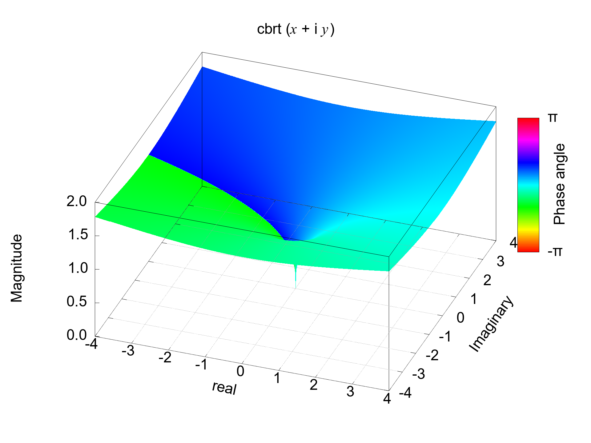
For the complex-valued version,
a different strategy is employed: the initial approximation is constructed by approximating the fractional exponent 1/3 through nested square roots,
effectively realizing expressions like xm/2n. This enables stable convergence across a broad dynamic range,
including both small and large magnitudes.
These methods are particularly suited for platforms where only square roots are natively supported or where minimizing operation latency is crucial,
offering a balance between simplicity, numerical stability, and performance.
The square root of x is given by x1/2 and The cube root of x is given by x1/3. When approximating the exponent 1/3 using the form m / 2n, where m = round(2n / 3), the approximation error is given by:
m / 2n × 3 - 1which results in an error of ±1/2n (with the negative sign when n is even). The specific values are:
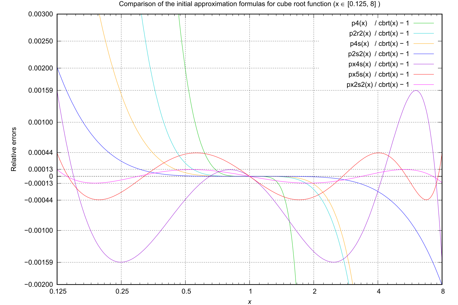
Among these, it was found that x11/32 is particularly suitable for achieving an initial approximation error of about half a digit, corresponding to a relative error of approximately ±1/√10 ≈ ±0.316, in the range [1e-10, 1e+10].1 / 2 × 3 - 1 = +0.5 1 / 4 × 3 - 1 = -0.25 3 / 8 × 3 - 1 = +0.125 5 / 16 × 3 - 1 = -0.0625 11 / 32 × 3 - 1 = +0.03125 21 / 64 × 3 - 1 = -0.015625 43 / 128 × 3 - 1 = +0.0078125 85 / 256 × 3 - 1 = -0.00390625
Fig.1: Approximation error when cube root x 1/3 is approximated by x m/2n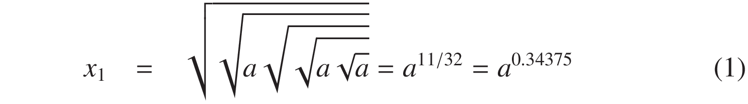
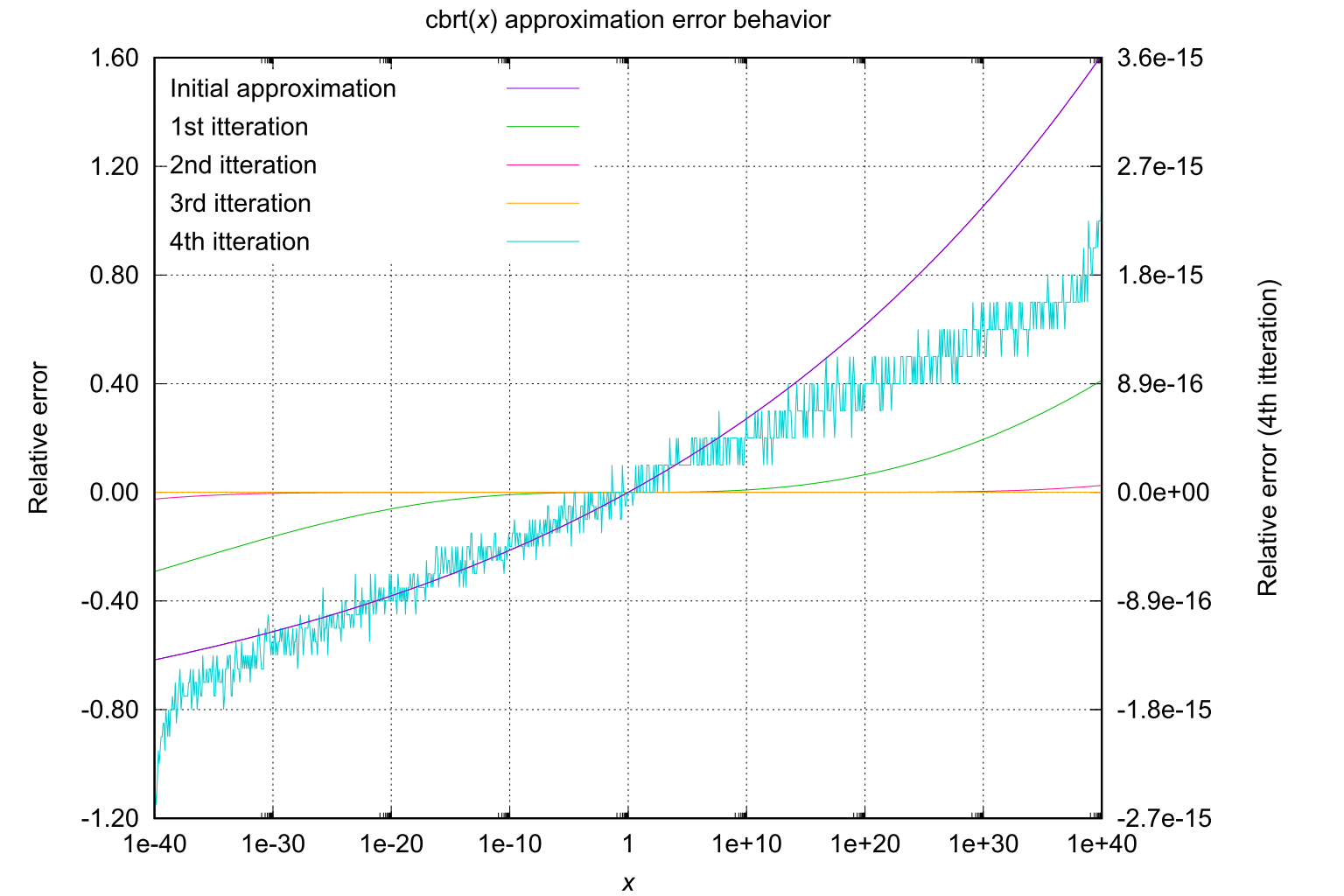
The maximum relative error of the initial approximation formula (1) over the range x ∈ [1e-12, 1e+12] is approximately +0.366 at x = 1e+12, which corresponds to a precision of about 0.437 decimal digits. Since the recurrence relation (6) described later exhibits cubic convergence, four iterations improve the precision by a factor of 3^4 = 81. Thus, the expected precision becomes:
0.437 × 81 ≈ 35.3 digits > 16 digits (IEEE 754 double precision)Therefore, double-precision accuracy can typically be achieved within four iterations.
Using the initial approximation obtained from equation (1), we refine the cube root using a recurrence relation similar to Newton's method.
Defining the relative error h as:![x = \sqrt[3]{a}](eqn-cbrt-a.png) The cube root function x1/3 can be expanded into an infinite series for x ≠ 0. Thus, we can express (1 + h)1/3 as the following series expansion:
The cube root function x1/3 can be expanded into an infinite series for x ≠ 0. Thus, we can express (1 + h)1/3 as the following series expansion: To obtain a more efficient iterative formula, we replace this series with a (1, 1) Padé approximation, which ensures that the first-order and second-order coefficients match those of the series expansion:
 From equations (3) and (5), we derive the following recurrence relation:

In the vicinity of the solution, Newton-Raphson iteration exhibits quadratic convergence. However, since the (1,1) Padé approximation matches the series expansion up to the second-order term, this recurrence relation achieves cubic convergence. Moreover, compared to the Newton-Raphson method, which can become unstable when the initial estimate is far from the true value, this Padé-based recurrence formula exhibits better numerical stability in such cases. Although the derivation process is different, the asymptotic formula is equivalent to that by Halley's method.
This method can be extended to the n-th root of a (where a ≠ 0), leading to the following asymptotic formula with cubic convergence:

Similarly to Equation (6), when using Padé approximants of order (2, 2) or (3, 3), the recurrence formulas (8) and (9) are obtained. These formulas exhibit fifth- and seventh-order convergence, respectively.


Fig.2: cbrt Initial approximatin error and its convergence behavior
(Computed under IEEE 754 Double precision environment)
Formulas usedInitial approximation :Recurrence formula of third order convergence :
Listing 1:
cbrt - for HP 42SListing 2:
ccbrt - complex cube root function in C9900 { 68-Byte Prgm } 01▸LBL "cbrt" 02 ABS 03 X=0? 04 RTN 05 LASTX 06 ENTER 07 ENTER 08 ENTER 09 SQRT 10 × 11 SQRT 12 SQRT 13 × 14 SQRT 15 SQRT 16▸LBL 00 17 ENTER 18 ENTER 19 X↑2 20 × 21 ENTER 22 + 23 LASTX 24 RCL+ ST T 25 RCL+ ST T 26 X<>Y 27 RCL+ ST T 28 ÷ 29 X<>Y 30 × 31 LASTX 32 RCL÷ ST Y 33 1 34 - 35 ABS 36 1?-11 37 X>Y? 38 GTO 01 39 R↓ 40 R↓ 41 GTO 00 42▸LBL 01 43 R↓ 44 R↓ 45 RTN 46 .END./* ccbrt Rev.1.5 (May 13, 2025) (c) 2003 Takayuki HOSODA * SPDX-License-Identifier: BSD-3-Clause * See https://opensource.org/licenses/BSD-3-Clause for details. */ /* REFERNCE ONLY: FOR EXPLANATION OF THE ALGORITHM AND NOT INTENDED FOR ACTUAL USE. */ #include <complex.h> #include <math.h> #include <float.h> double complex ccbrt(double complex x); /* The ccbrt(x) function compute the cube root of x. */ double complex ccbrt(double complex a) { double complex x, xp, c; double r, rp, s; int e; if (a == 0) return 0; /* Simple range reduction */ #ifdef USE_FREXP frexp(cabs(a), &e); x = a * ldexp(1.0, -e + e % 3); s = ldexp(1.0, e / 3); #else x = a; s = 1.0; while (cabs(x) < 0x1.0p-195) { x *= 0x1.0p+195; s *= 0x1.0p-65; } while (cabs(x) > 0x1.0p+195) { x *= 0x1.0p-195; s *= 0x1.0p+65; } while (cabs(x) < 0x1.0p-39) { x *= 0x1.0p+39; s *= 0x1.0p-13; } while (cabs(x) > 0x1.0p+39) { x *= 0x1.0p-39; s *= 0x1.0p+13; } #endif /* Initial approximation by x^(11/32) and range expansion */ x = csqrt(csqrt(x*csqrt(csqrt(x*csqrt(x))))) * s; r = 0x1.0p+39; do { /* Asymptotic formula */ xp = x; rp = r; c = x * x * x; #if defined( USE_SEVENTH ) x += x * (a - c) * (5 * (a * a + c * c) + 17 * a * c ) / (a * a * (a + a + 30 * c) + c * c * (42 * a + 7 * c)); #elif defined( USE_FIFTH ) x += 9 * x * (a + c) * (a - c) / (14 * c * c + 35 * a * c + 5 * a * a); #else x += x * (a - c) / (c + c + a); /* Cubic convergence */ #endif r = cabs(x - xp); /* Correction radious */ } while (r != 0 && rp > r); /* Convergence check by Urabe's method */ return x; }Note: Practical use may require exception handling and range reduction.
Download : cbrt.raw — (raw program file for Free42)
In the case of real numbers, if your environment supports the sqrt function along with ldexp and frexp for directly manipulating the exponent part of floating-point numbers, range reduction becomes straightforward. Using a Puiseux-series-like approximation based on powers of 1/2 (i.e., square roots), we present the following 3-term initial approximation formula (10), optimized for the range reduced to [0.125, 4]:
The maximum approximation error of the initial formula (10) is approximately 0.009, which corresponds to about 2.04 decimal digits of precision. Therefore, applying the previously discussed recurrence formula (6) of third-order convergence twice gives: 2.04 × 32 = 18.4 digits of precision, which is sufficient to achieve IEEE 754 double-precision accuracy.
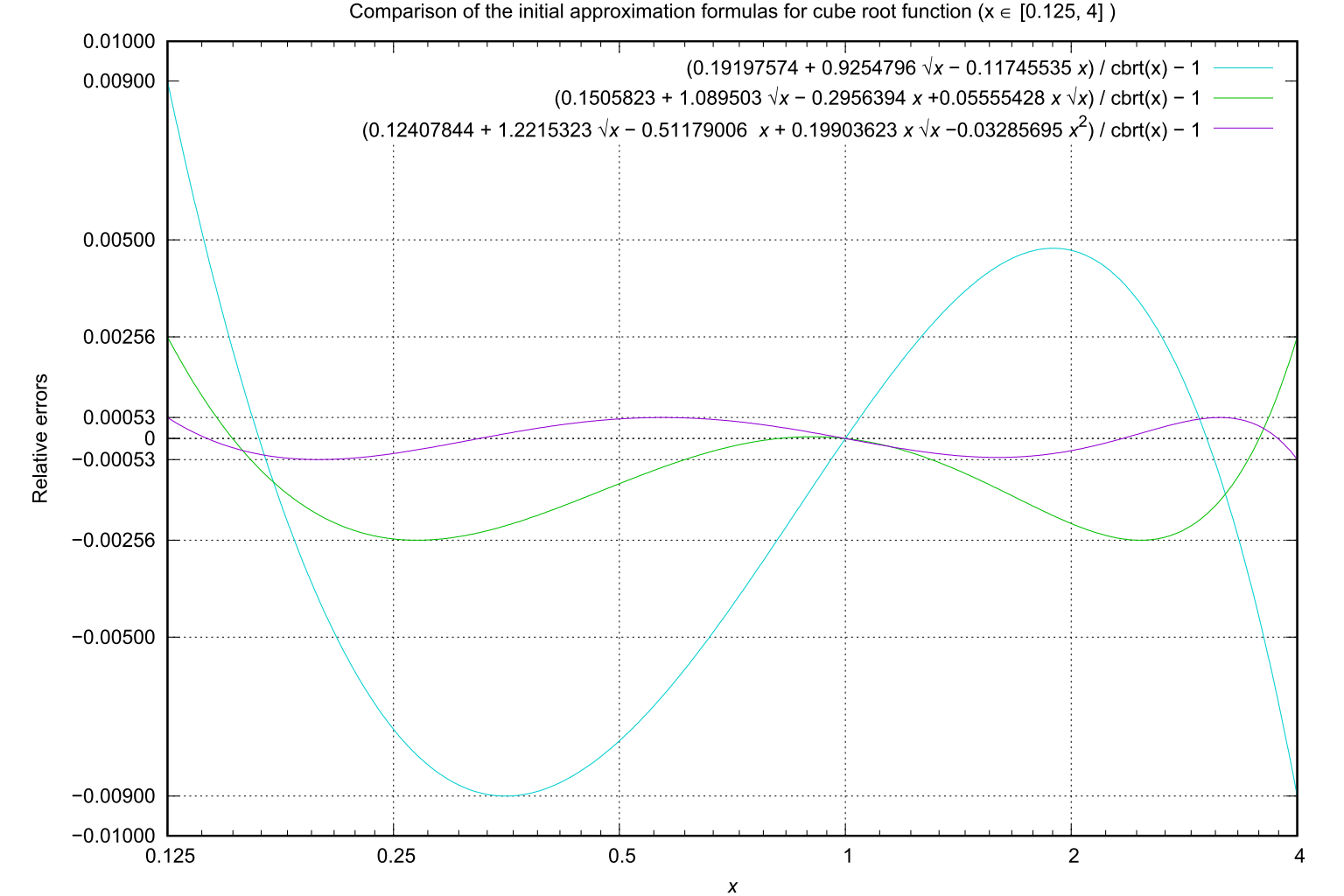
Fig.3: Approximation error in cube root estimation using 3- to 5-term expressions involving square roots (x ∈ [0.125, 4])
If formula (10) is used in 80-bit extended precision arithmetic (such as the x87 floating-point format), applying the cubic-converging recurrence formula (6) twice is not sufficient to reach the full precision of approximately 19 decimal digits. In such cases, the following 4-term initial approximation formula (11), which is optimized over the interval [0.125, 4], provides improved accuracy. The maximum relative error of this approximation is approximately 0.00256, corresponding to a precision of about 2.59 decimal digits. Thus, applying the same cubic-converging recurrence formula (6) twice yields:
2.59 × 32 ≈ 23.3 digits > 19 digits (extended precision)and hence allows the desired accuracy to be achieved.
Listing 3:
_cbrt - cube root function in C89 (ANSI-C)/* _cbrt Rev.2.3 (May 7, 2025) (c) 2025 Takayuki HOSODA * SPDX-License-Identifier: BSD-3-Clause * See https://opensource.org/licenses/BSD-3-Clause for details. */ #include <math.h> #include <float.h> double _cbrt(double d); /* The _cbrt(d) function compute the cube root of d.*/ double _cbrt(double d) { double r, x, a, c; int e; if (d == 0) return 0; r = frexp(fabs(d), &e); /* Range reduction: r is in [0.5, 1.0) */ x = ldexp(r, e % 3); /* x is in [0.125, 4) */ /* Initial approximation formula for x in [0.125, 4] with |err| < 0.00256 */ a = 0.1505823 + 1.089503 * sqrt(x) - 0.2956394 * x + 0.0555543 * x * sqrt(x); /* Apply the asymptotic formula of cubic convergence twice */ c = a * a * a; a += a * (x - c) / (c + c + x); c = a * a * a; a += a * (x - c) / (c + c + x); #ifndef OMIT_ADJ /* A 1-ulp correction to ensure result consistency. */ if (a * a * a * (1.0 - DBL_EPSILON) > x) a *= (1.0 - 0.5 * DBL_EPSILON); if (a * a * a * (1.0 + 2.0 * DBL_EPSILON) < x) a *= (1.0 + DBL_EPSILON); #endif return ldexp(d > 0.0 ? a : -a, e / 3); /* Return with range expansion */ }
Listing 4:
_cbrtl - cube root function in C89 (ANSI-C)/* _cbrtl Rev.2.3 (May 7, 2025) (c) 2025 Takayuki HOSODA */ * SPDX-License-Identifier: BSD-3-Clause * See https://opensource.org/licenses/BSD-3-Clause for details. */ #include <math.h> #include <float.h> long double _cbrtl(long double d); /* The _cbrtl(d) function compute the cube root of d.*/ long double _cbrtl(long double d) { long double r, x, a, c; int e; if (d == 0) return 0; r = frexpl(fabsl(d), &e); /* Range reduction: r is in [0.5, 1.0) */ x = ldexpl(r, e % 3); /* x is in [0.125, 4) */ /* Initial approximation formula for x in [0.125, 4] with |err| < 0.00256 */ a = 0.1505823 + 1.089503 * sqrtl(x) - 0.2956394 * x + 0.0555543 * x * sqrtl(x); /* Apply the asymptotic formula of cubic convergence twice */ c = a * a * a; a += a * (x - c) / (c + c + x); c = a * a * a; a += a * (x - c) / (c + c + x); #ifndef OMIT_ADJ /* A 1-ulp correction to ensure result consistency. */ if (a * a * a * (1.0 - LDBL_EPSILON) > x) a *= (1.0 - 0.5 * LDBL_EPSILON); if (a * a * a * (1.0 + 2.0 * LDBL_EPSILON) < x) a *= (1.0 + LDBL_EPSILON); #endif return ldexpl(d > 0.0 ? a : -a, e / 3); /* Return with range expansion */ }Note:
In an empirical evaluation conducted using GCC 7.5, the custom _cbrt and _cbrtl functions were tested on 1,000,000 randomly generated double-precision and long double-precision values, respectively. The relative error, computed as_cbrt(d)3 / d - 1and_cbrtl(d)3 / d - 1, was found to be within ±4.44089209850063e-16 and ±2.16840434497101e-19, approximately twice the machine epsilon for IEEE 754 double and long double precision, respectively.Both _cbrt(d) and _cbrtl(d) also support negative arguments: for
d < 0, they return-_cbrt(-d)and-_cbrtl(-d), respectively, consistent with the fact that the cube root, being an odd-degree root, is continuously defined over the entire set of real numbers.
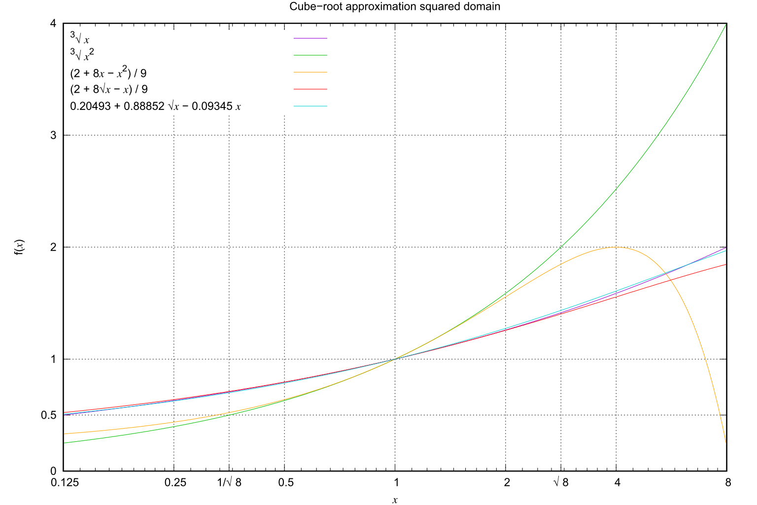
In the implementation example of the real-valued cube root, we used Equation (10), which includes square root terms, as the initial approximation. This approximation was designed based on the following idea:
We begin by constructing a Padé approximation of order (2, 0) is applied to the cube root of x2 around x ≈ 1.
Then, by substituting x with √x in in place of x in the resulting expression, we obtain an approximation for the cube root of x itself.
This transformation effectively squares the domain of approximation, thereby expanding the region over which the cube root approximation maintains a low error.
Figure 4 shows an example in which the resulting expression was adjusted to satisfy cbrt(1) = 1, while minimizing the maximum absolute approximation error over the interval x ∈ [0.125, 8]
Equation (10) was similarly optimized over the interval x ∈ [0.125, 4] to be used withfrexpandldexpfunctions in C.
Fig.4: Approximation of cube root over the squared domain (x ∈ [0.125, 8])
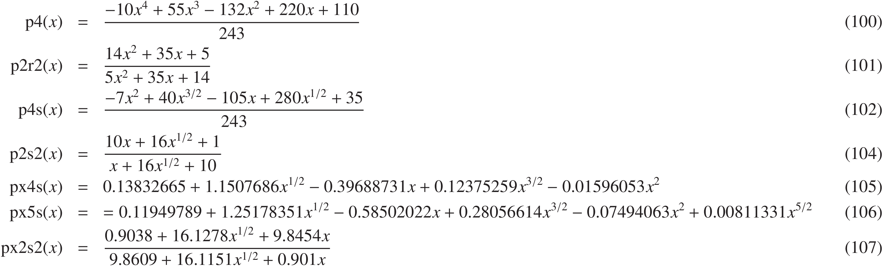
As a reference, several higher-order approximation formulas designed with the same idea are presented below, along with a comparison graph.
These formulas approximate the cube root using 4- to 5-term series expansions that include square root terms.
Approximation formulas:
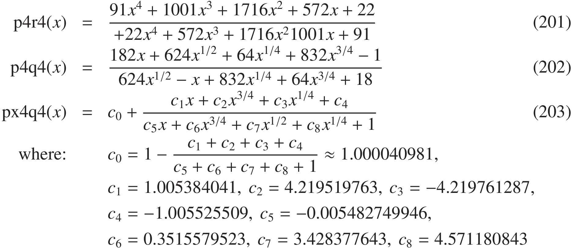
As a further extension of the methods described above, we present below a design example of a highly accurate initial approximation.
First, the (4, 4) Padé approximation formula (201) for cube roots demonstrates,
through numerical evaluation, a precision of more than 7.6 decimal digits within the range x ∈ [1/4√8, 4√8].
In contrast, formula (202), which is constructed based on a Padé approximation for the 3/4 power root,
achieves a comparable level of precision over the expanded range x ∈ [0.125, 8], corresponding to a range enlargement by a factor of approximately 83/4 ≈ 4.76.
Furthermore, formula (203), derived by optimizing the coefficients of formula (202),
achieves more than 9.0 digits of accuracy over the same range.
For example, compared to the somewhat more primitive approximation formula (105),
formula (203) increases the number of division and square root operations by one each,
yet demonstrates a substantial improvement in accuracy from approximately 1.8 digits to 9.0 digits over x ∈ [0.125, 8] (see Fig.6).
Thus, the ability to achieve practically sufficient accuracy of more than 9 digits using only the initial approximation—without the need for convergence checks, conditional branching,
or iterative methods such as Newton's method—makes this approach highly valuable for industrial applications such as real-time control, where minimizing computation time variability is crucial.
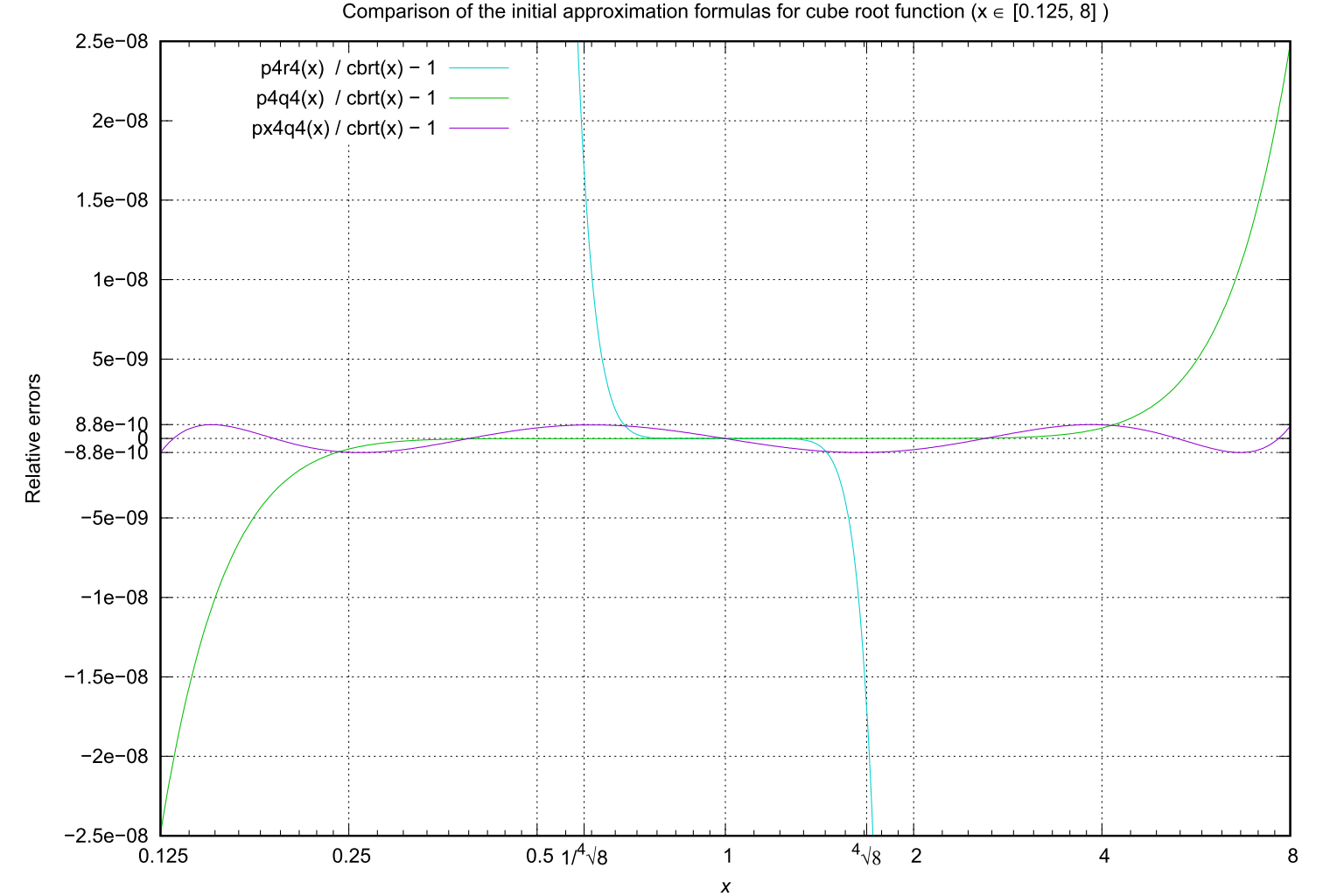
Fig.6: Approximation error of the cube root using an 8-term expansion involving the fourth root (x ∈ [0.125, 8])
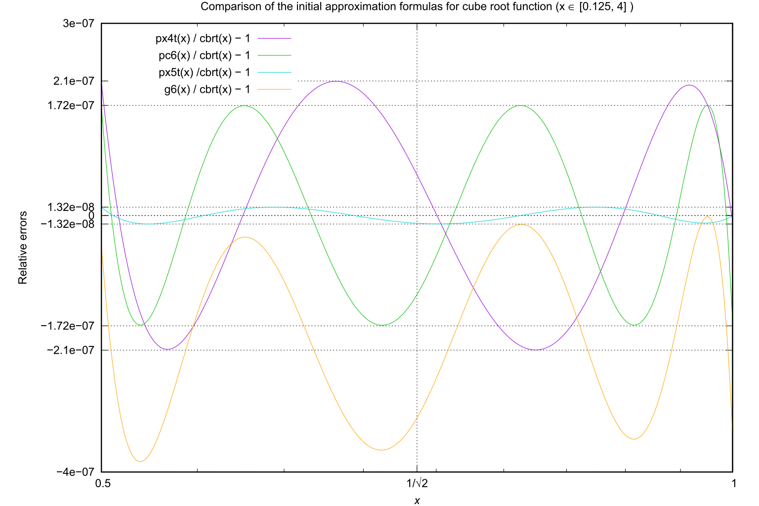
As a practical reference, the following is an example of a cube root function in C that avoids the use of square roots, and instead employs a 6th-degree Minimax polynomial approximation as the initial estimate. This approximation (Equation (301)) achieves an accuracy of 6.7 decimal digits over the interval x ∈ [0.5, 1]. When used as an initial guess for a single iteration of Halley's method, it theoretically yields 20.2-digit precision, which meets the precision of the IEEE 754
Approximation formulas:double(orlong double) format. An additional ULP-level correction is applied after the approximation to improve robustness. On processors equipped with multiple pipelines and fused multiply-add (FMA) units, this method may outperform the previously discussed_cbrtfunction that uses square roots.
![\mathrm{pc6}(x) &=& \sum_{k=0}^6 c_k x^k, \quad x \in [0.5, 1] &(301)\\
\text{where:}
&& c_0 = 0.35489555,\ c_1 = 1.50819458,\\
&& c_2 = -2.11500172,\ c_3 = 2.44693876,\\
&& c_4 = -1.83469500,\ c_5 = 0.78493037,\\
&& c_6 = -0.14526271&\\
\mathrm{px4t}(x)&=& \sum_{k=0}^4 c_k x^{k/2}, \quad x \in [0.5, 1] &(302)\\
\text{where:}
&& c_1 = 0.1284692,\ c_2 = 1.21926614,\\
&& c_3 = -0.540296,\ c_4 = 0.2422709,\\
&& c_5 = -0.04971025\\
\mathrm{px5t}(x) &=& \sum_{k=0}^5 c_k x^{k/2}, \quad x \in [0.5, 1] &(303)\\
&& c_1 = 0.11132305,\ c_2 = 1.32115104,\\
&& c_3 = -0.78151144,\ c_4 = 0.52669338,\\
&& c_5 = -0.21674025,\ c_6 = 0.03908422\\](eqn-cbrt-c6.png)
Fig.7: Approximation error of a 6th-degree polynomial Minimax approximation of the cube root (x ∈ [0.5, 1])
Listing 5:
h_cbrt - cube root function in C89 (ANSI-C)/* h_cbrt Rev.1.0 (May 7, 2025) Copyright (c) 2025 Takayuki HOSODA * SPDX-License-Identifier: BSD-3-Clause * See https://opensource.org/licenses/BSD-3-Clause for details. */ #include <math.h> #include <float.h> long double h_cbrtl(long double x); /* The h_cbrt(x) function compute the cube root of x. */ double h_cbrt(double x) { double a, b, c, d, t; int e; static const double scf[5] = { 0.62996052494743658238361, /* 1 / cbrt(4) */ 0.79370052598409973737585, /* 1 / cbrt(2) */ 1.0, 1.25992104989487316476721, /* cbrt(2) */ 1.58740105196819947475171 /* cbrt(4) */ }; if (x == 0) return 0; d = frexp(a = fabs(x), &e); /* d is in [0.5, 1) */ t = d * d; b = 0.78493037; c = - 0.14526271; b = b * t + 2.44693876; c = c * t - 1.83469500; b = b * t + 1.50819458; c = c * t - 2.11500172; b = b * d + 0.35489555; c = c * t + b; /* |error| < 1.715e-7 */ t = c * c * c; b = scf[2 + e % 3]; c = (c + c * (d - t) / (2 * t + d)) * ldexp(b, e / 3); if ((c * c * c) * (1 - DBL_EPSILON) > a) c *= (1 - 0.5 * DBL_EPSILON); if ((c * c * c) * (1 + 2 * DBL_EPSILON) < a) c *= (1 + DBL_EPSILON); return x > 0.0 ? c : -c; }
Listing 6:
h_cbrtl - cube root function in C89 (ANSI-C)/* h_cbrtl Rev.1.0 (May 8, 2025) (c) 2025 Takayuki HOSODA * SPDX-License-Identifier: BSD-3-Clause * See https://opensource.org/licenses/BSD-3-Clause for details. */ #include <math.h> #include <float.h> long double h_cbrtl(long double x); /* The h_cbrtl(x) function compute the cube root of x. */ long double _cbrtl(long double x) { long double a, b, c, d, t; int e; static const long double scf[5] = { 0.62996052494743658238361L, /* 1 / cbrt(4) */ 0.79370052598409973737585L, /* 1 / cbrt(2) */ 1.0L, 1.25992104989487316476721L, /* cbrt(2) */ 1.58740105196819947475171L /* cbrt(4) */ }; if (x == 0) return 0; d = frexpl(a = fabsl(x), &e); /* d is in [0.5, 1) */ t = d * d; b = 0.78493037; c = - 0.14526271; b = b * t + 2.44693876; c = c * t - 1.83469500; b = b * t + 1.50819458; c = c * t - 2.11500172; b = b * d + 0.35489555; c = c * t + b; /* |error| < 1.715e-7 */ t = c * c * c; b = scf[2 + e % 3]; c = (c + c * (d - t) / (2 * t + d)) * ldexpl(b, e / 3); if ((c * c * c) * (1 - LDBL_EPSILON) > a) c *= (1 - 0.5 * LDBL_EPSILON); if ((c * c * c) * (1 + 2 * LDBL_EPSILON) < a) c *= (1 + LDBL_EPSILON); return x > 0.0 ? c : -c; }Note:
In an empirical evaluation conducted using GCC 7.5, the custom h_cbrt and h_cbrtl functions were tested on 1,000,000 randomly generated double-precision and long double-precision values, respectively. The relative error, computed ash_cbrt(d)3 / d - 1andh_cbrtl(d)3 / d - 1, was found to be within ±4.44089209850063e-16 and ±2.16840434497101e-19, approximately twice the machine epsilon for IEEE 754 double and long double precision, respectively.
The previously presented cube root function that avoids using
sqrtmay appear lightweight; however, its initial approximation involves a relatively high number of polynomial terms. This results in a large number of constant loads and fused multiply-add (FMA) operations, which can limit performance improvements, especially on architectures where instruction throughput is a bottleneck.In contrast, by narrowing the approximation domain to x ∈ [0.5, 1], the square-root-based method can achieve comparable accuracy with fewer terms, which may lead to better performance on modern processors with efficient floating-point units.
For example, Equation (301) achieves an initial approximation accuracy of approximately 6.8 digits using 7 polynomial coefficients, while Equation (302), which incorporates square roots, attains about 6.7 digits with only 5 coefficients (see Fig. 7).
The following is a C implementation of the cube root function using this square-root-based initial approximation.
Listing 7:
q_cbrt - cube root function in C89 (ANSI-C)/* q_cbrt Rev.1.0 (May 9, 2025) (c) 2025 Takayuki HOSODA * SPDX-License-Identifier: BSD-3-Clause * See https://opensource.org/licenses/BSD-3-Clause for details. */ #include <math.h> #include <float.h> double q_cbrt(double x); /* The q_cbrt(x) function compute the cube root of x. */ double q_cbrt(double x) { double a, b, c, d, t; int e; static const double scf[5] = { 0.62996052494743658238361, /* 1/cbrt(4) */ 0.79370052598409973737585, /* 1/cbrt(2) */ 1.0, 1.25992104989487316476721, /* cbrt(2) */ 1.58740105196819947475171 /* cbrt(4) */ }; if (x == 0) return 0; d = frexp(a = fabs(x), &e); /* d is in [0.5, 1] */ c = 0.12846922 - (0.54029596 + 0.0497103 * d) * d + (1.2192661 + 0.24227096 * d) * sqrt(d); /* |err| < 2.1e-7 */ b = scf[2 + e % 3]; t = c * c * c; c = (c + c * (d - t) / (2 * t + d)) * ldexp(b, e / 3); if ((c * c * c) * (1 - DBL_EPSILON) > a) c *= (1 - 0.5 * DBL_EPSILON); if ((c * c * c) * (1 + 2 * DBL_EPSILON) < a) c *= (1 + DBL_EPSILON); return x > 0.0 ? c : -c; }
Listing 8:
q_cbrtl - cube root function in C89 (ANSI-C)/* q_cbrtl Rev.1.0 (May 9, 2025) (c) 2025 Takayuki HOSODA * SPDX-License-Identifier: BSD-3-Clause * See https://opensource.org/licenses/BSD-3-Clause for details. */ #include <math.h> #include <float.h> long double q_cbrtl(long double x); /* The q_cbrtl(x) function compute the cube root of x. */ long double q_cbrtl(long double x) { long double a, b, c, d, t; int e; static const long double scf[5] = { 0.62996052494743658238361L, /* 1/cbrt(4) */ 0.79370052598409973737585L, /* 1/cbrt(2) */ 1.0, 1.25992104989487316476721L, /* cbrt(2) */ 1.58740105196819947475171L /* cbrt(4) */ }; if (x == 0) return 0; d = frexpl(a = fabsl(x), &e); /* d is in [0.5, 1] */ c = 0.12846922 - (0.54029596 + 0.0497103 * d) * d + (1.2192661 + 0.24227096 * d) * sqrtl(d); /* |err| < 2.1e-7 */ b = scf[2 + e % 3]; t = c * c * c; c = (c + c * (d - t) / (2 * t + d)) * ldexpl(b, e / 3); if ((c * c * c) * (1 - LDBL_EPSILON) > a) c *= (1 - 0.5 * LDBL_EPSILON); if ((c * c * c) * (1 + 2 * LDBL_EPSILON) < a) c *= (1 + LDBL_EPSILON); return x > 0.0 ? c : -c; }
Note:
In an empirical evaluation conducted using GCC 7.5, the custom h_cbrt and h_cbrtl functions were tested on 1,000,000 randomly generated double-precision and long double-precision values, respectively. The relative error, computed ash_cbrt(d)3 / d - 1andh_cbrtl(d)3 / d - 1, was found to be within ±4.44089209850063e-16 and ±2.16840434497101e-19, approximately twice the machine epsilon for IEEE 754 double and long double precision, respectively.
Function Under Test Relative error Execution time Note n=1000000 n=10000000 min max cputime [s] cbrt (Ref.#1) -5.55E-16 6.66E-16 0.187500 libm, system dependent __cbrt (Ref.#2) -1.55E-15 2.00E-15 0.250000 glibc-2.41, ieee754/dbl-64/s_cbrt.c q_cbrt -1.22E-15 6.66E-16 0.210938 OMIT_ADJ h_cbrt -1.22E-15 6.66E-16 0.218750 OMIT_ADJ r_cbrt -6.66e-16 6.66E-16 0.359375 OMIT_ADJ q_cbrt -4.44E-16 4.44E-16 0.242188 cf. Listing 7 h_cbrt -4.44E-16 4.44E-16 0.250000 cf. Listing 5 r_cbrt -4.44E-16 4.44E-16 0.437500 cf. Listing 3 cbrtl -3.25E-19 3.25-19 0.390625 80-bit long double, libm, system dependent q_cbrtl -2.17E-19 2.17E-19 0.414062 80-bit long double, cf. Listing 8 h_cbrtl -2.17E-19 2.17E-19 0.421875 80-bit long double, cf. Listing 6 r_cbrtl -2.17E-19 2.17E-19 0.648438 80-bit long double, cf. Listing 4 CPU: Intel(R) Xeon(R) CPU E3-1220 V2 @ 3.10GHz (3093.04-MHz K8-class CPU) CC: gcc7.5.0 -O2 -march=native
This article has explored a method for approximating the cube root using only square roots, along with implementation examples. For the initial approximation, a Puiseux-like expansion was used in the real-valued version, and an exponential form xm/2n was used in the complex-valued version, followed by a Padé-type iterative refinement to improve accuracy.
The proposed approximations and iterative methods, while relatively simple in form, demonstrated good convergence and accuracy for both real and complex inputs. Since the computational cost of evaluating square roots is comparable to that of division, the approaches presented here, though not widely established, may serve as practical options for cube root computation.
Further research into higher-order initial approximations and comparisons with alternative iterative methods may lead to even higher precision or faster algorithms in the future.
Note: The initial approximation method for cube roots described in this article — namely, constructing a Pade approximation of x 2/3 near x = 1, then substituting x with √x to transform it into a function of x 1/3, thereby expanding the effective approximation range — is a technique independently developed by the author based on the idea of Puiseux series. As of the time of writing, no similar approach has been found in the literature.
Usage of cbrt (HP 42S)OperationCalculation example of cbrt (HP 42S)Input
Output
 2 "cbrt" → 1.25992104989
-3 "cbrt" → 0.72112478515 + 1.24902476648 i
0 ENTER 1 COMPLEX "cbrt" → 0.866025403784 + 0.5 i
0 ENTER 10 COMPLEX "cbrt" → 1.86579517236 + 1.07721734502 i
-16 ENTER 16 COMPLEX "cbrt" → 2 + 2 i
1e9 ENTER "cbrt" → 1000

![[Mail]](/~lyuka/images/mail.gif)


 © 2000 Takayuki HOSODA.
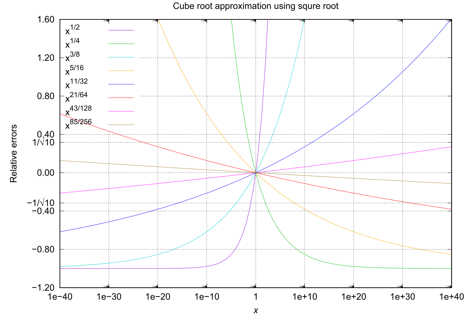
![x_0 &=& c_1 + c_2 a^{1/2} + c_3 a + c_4 a^{3/2}, \quad x \in [0.125, 4] &\\
\text{where:}&& c_1= 0.1505823,\quad c_2 = 1.089503,\\
&& c_3 = - 0.2956394,\ c_4 = 0.0555543](eqn-cbrt-px4n.png)