An example of Bessel filter calculation and
Inverse Bessel polynomial roots by the DKA (Durand-Kerner-Aberth) method
Takayuk HOSODA
Apr. 11, 2024

It is now spring 2024, and Generative Pre-trained Transformers and cherry blossoms are in full bloom, I found a design table of active filters in the handbook of a technical magazine supplement. I know that flowers and GPTs are for viewing and not for use, but I was concerned because the design values for the Bessel filter [1][2] in the numerical table seemed to be "slightly" different.
I don't want to be serendipitous about it, but I was curious and did a bit of research. I couldn't trace the source of the table, but it seems to match the published values by about five digits when compared with the values calculated with the strict -3 dB cut-off frequency instead of √0.5, which seems like a total oversimplification (*1) The reason for about five digits is that the dawn of modern network theory in Japan was in the 1950s, and the original calculations may have been due to the single precision of the available computing environment.
In actual circuit design, pure Bessel filters are rarely employed, and even if they were, it is rare to design from a table of numbers now that a variety of design applications are available. However, there are also cases where a Bessel filter is required in terms of mathematical understanding and intrinsic nature, even if it is not a Bessel filter itself, from the point of view of error rates and EMC. For these reasons, this is a good opportunity to summarise the calculation examples, calculation programs and design tables for Bessel filters once again.
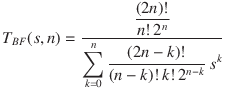
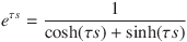
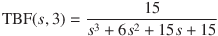
The transfer function of a third-order Bessel filter TBF(s, 3) can be approximated by a serial fraction expansion of the time delay transfer function [2][3] as follows
The cut-off frequency fc at which the absolute value of the amplitude of TBF(s, 3) is 1 / √2 is calculated as follows
fc = solve(abs(TBF(s, 3), s) - sqrt(0.5) → fc ≃ 1.75567236868121064920
Where solve(f(s), s) means solve (*2) the function f(s) for s.
The normalised transfer function TBFN(s, 3) of the third-order Bessel filter normalised by fc approximately becomes

The poles p of TBFN(s, 3) are obtained by solving the denominator as follows.
solve(15 / TBFN(s, 3), s) → p ≃ {-1.322675800, -1.047409161 ± i 0.9992644365 }
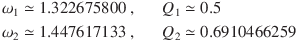
The natural frequency ω and quality factor Q for one pole p of p are defined as follows

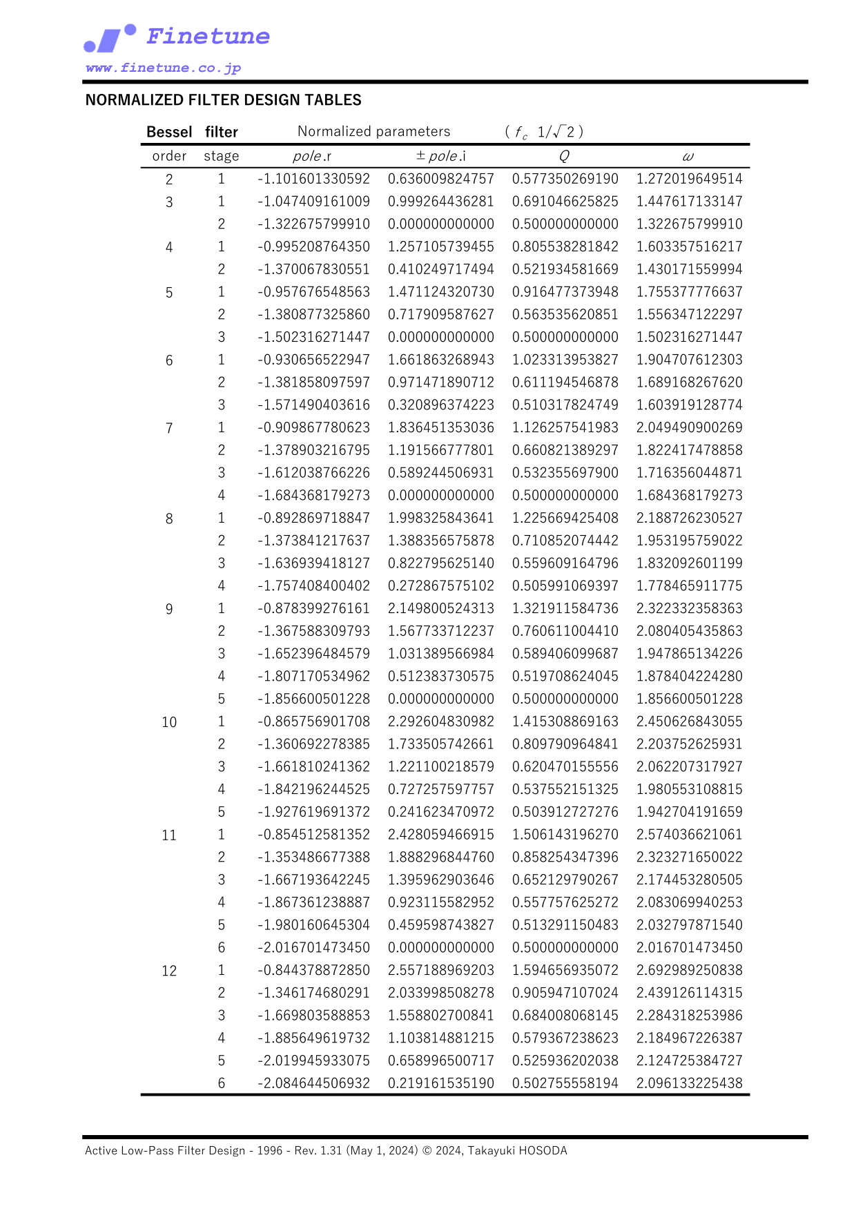
Therefore, the normalised design parameters for a third-order Bessel filter in a two-stage configuration are calculated as follows
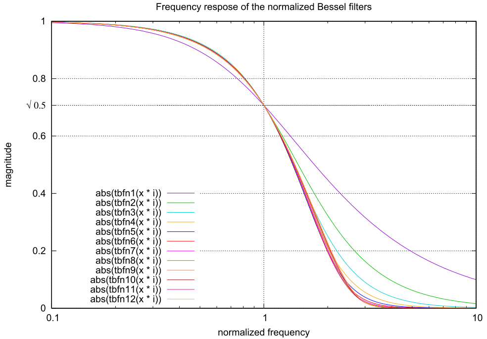
Frequency versus amplitude characteristics of the normalised Bessel filters (1st to 12th order)
fig.1 Frequency response of the normalized Bessel filters (1st - 12th order)Results of SPICE3 simulations of the normalised Bessel filters (1st to 12th order)
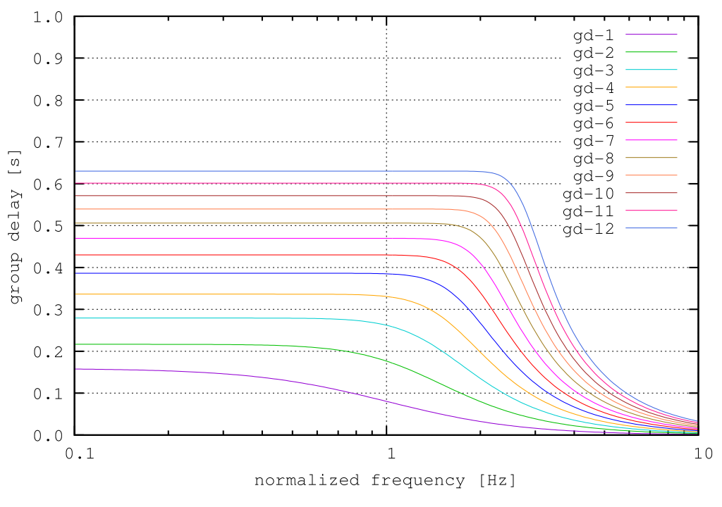
fig.2 Group delay characteristics of the normalized Bessel filters (1st to 12th order)
AC simulation results of the normalised Bessel filter of active filters with ideal op-amps using SPICE3.
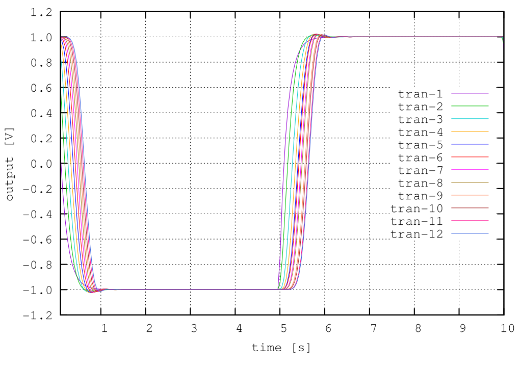
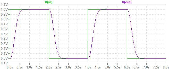
fig.3 Transcient response of the normalized Bessel filters (1st to 12th order)
TRAN simulation results of the normalised Bessel filter of active filters with ideal op-amps using SPICE3.
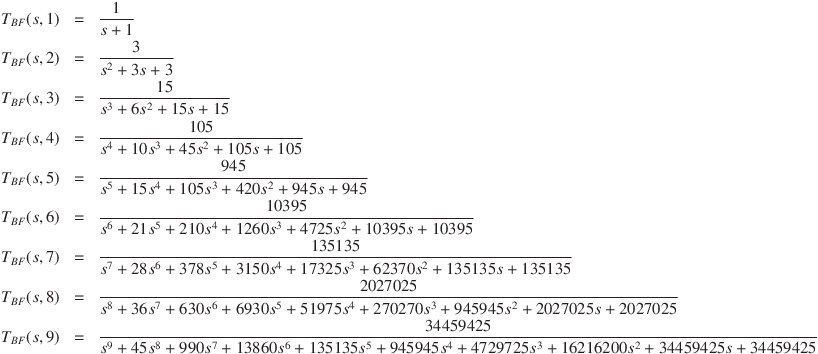
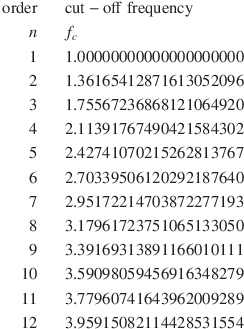
The transfer function of the Bessel filters (1st to 12th order)

The cut-off frequency of the Bessel filters (1st to 12th order)
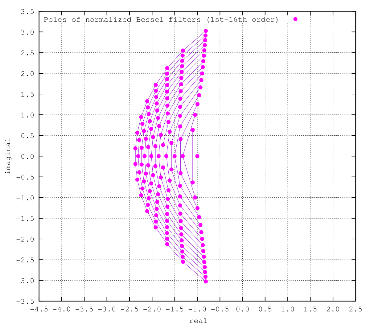
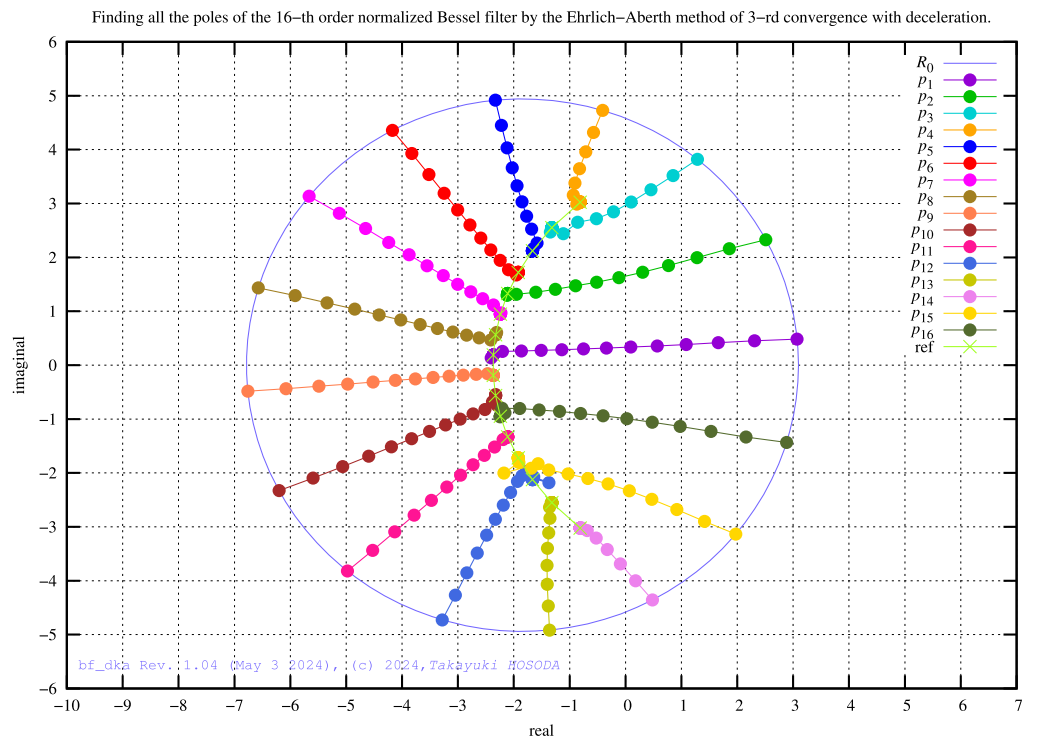
Poles of the normalised Bessel filter (2nd to 12th order)
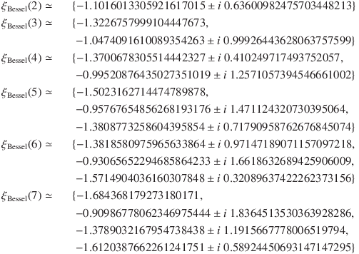
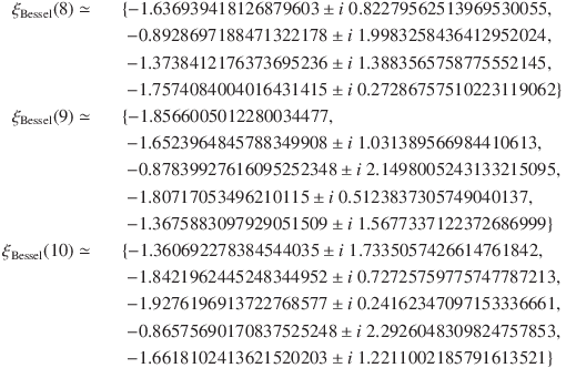
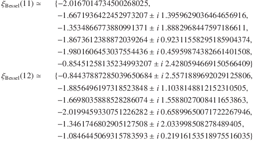
fig.4 Poles of the normalized Bessel filters (1st - 16th order)
Poles are connected by lines for each group.
Source code (C99)
bf_dka -- A solver for reverse Bessel polynomials using the Durand-Kerner-Aberth method.

bf_dka_xp_mini-1.21.tar.gz— C source code for a minimal version of bf_dka for educational purposes. Can be compiled under *BSD or Linux.
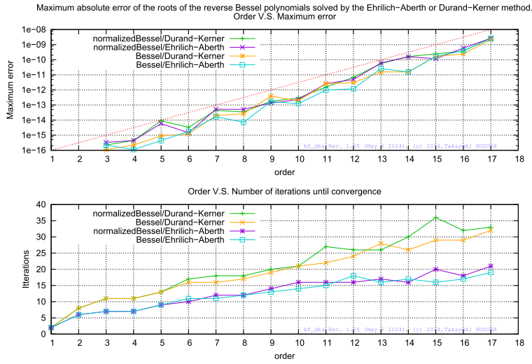
I tried to find some textbooks and practical books related to analogue filters, but... I haven't been able to find an "accurate" table of 8+ digit numbers with a basis for calculations. There are a number of excellent CAS (Computer Algebra Systems) available nowadays, but I tried again to see how far I could get with 64-bit integers and C99 double-precision complex or extended-precision complex numbers. Unlike CAS, when you write in C, you can keep all the algorithms and optimisations for the limits of the computer in your hands, so I'm glad to be able to use it for other purposes. The results of the above program using the Durand-Kerner-Aberth (DKA) method in x86 extended-precision were valid up to 14 digits at 12th order, 12 digits at 16th order and 8 digits at 17th order in comparison with the reference value which was calculated to 25 digits of precision in CAS (c.f. fig.5). For the double precision version not listed here, 11 digits were valid up to the 12th order, 9 digits up to the 16th order and 8 digits up to the 17th order (c.f. fig.6).
fig.5 Maximum error V.S. order (Ehrilich-Aberth and Durand-Kerner method, x86 extended precision)
fig.6 Maximum error V.S. order (Ehrilich-Aberth and Durand-Kerner method, double precision)
*1 : By definition, the cut-off frequency is the frequency at which the transferred power is halved, since it is
1/√2 ≃ -3 dB (i.e. 10-3/20 / (1/√2) - 1 ≃ 0.0011865297 ). In radio engineering, an error of about 0.1 % is negligible, but in the case of numerial tables it is a different story.*2 : The Newton-Raphson method, Ostrowski's method [4][5] and others are used for solving equations, DKA (Durand-Kerner-Aberth) method [4] [6] [9] and others are used for solving higher-order algebraic equations.
Design table for normalised Bessel filters (2nd to 17th order)
normalized-Bessel-filter-design-parameters-1.31.pdf
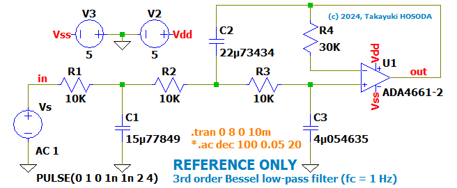
Bessel filter simulation circuit example (3rd order, VCVS type, for LTspice)
bessel3-ltspice.zip
- G.N.Watson. A TREATISE ON THE THEORY OF BESSEL FUNCTIONS. SECOND EDITION. Cambridge University Press, 1966, 815p
- Thomson, W.E. "Delay networks having maximally flat frequency characteristics", Proceedings of the IEE - Part III: Radio and Communication Engineering, 1949, 96, (44), p. 487-490
- Akio Katsumada "About the automatic design of Bessel digital filters" Seismic Test Report Vol. 56, 1993, p. 17-34
- Hayato Togawa "Scientific and Technical Computing Handbook", Science Publishing, Tokyo, 1992, ISBN 4-7819-0666-4
- .M.Ostrowskis. SOLUTION OF EQUATIONS IN EUCLIDEAN AND BANACH SPACES. THIRD EDITION. Academic Press, New Yoark and London, 1973
- Tetsuro Yamamoto, Utaro Furukane, Kumi Nokura "Durand-Kerner method and Aberth method for solving algebraic equations", Information Processing Vol.18 No.6 June 1977, p. 566-571
- Tsuneo Shiraki, Takao Terano, Hideharu Nakamura, and Chizuko Kurihara, "Solution of transcendental equations using the DKA method and its application examples," Proceedings of the Japan Society of Civil Engineers, No. 416/1-13, 1990, p. 295-302
- Edited by Ryo Natori, co-authored by Hidehiko Hasegawa, Tetsuya Sakurai, Sumiko Hiyama, et al., "Numerical Calculation Method", Ohmsha, Tokyo, Japan, 1998.9, p.109-113, ISBN 4-274-13153-X
- Kazufumi Ozawa, "Simple method for setting efficient initial values ??of the Durand-Kerner method", Transactions of the Japan Society of Applied Mathematics Vol.3, No.4, 1993, p.173-186
- Anatol I. Zverev, "Handbook of Filter Synthesis", John Wiley and Sons, Inc, New York London Sydney, 1967, p. 61-71
- BesselFilterModel — WOLFRAM
- Bessel analog filter design — MathWorks
- Gershgorin Circle Theorem — Wolfram MathWorld
- Bessel filter — Wikipedia
- Pade approximant — Wikipedia
- Spice — a circuit simulator / UC Berkeley
- LTspice — free SPICE simulator software / Analog Devices / Linear Technology
- gnuplot — graphing utility
- GCC — the GNU Compiler Collection

![[Mail]](/~lyuka/images/mail.gif)


 © 2000 Takayuki HOSODA.